June 2013

You are currently browsing the monthly archive for June 2013.

Robin Hanson gave a very interesting TED talk about a possible technological singularity based on AI and robotics.  I outline his talk below and add a few ideas from Hanson’s 1998 article “Long-Term Growth As A Sequence of Exponential Modes“, Ray Kurzweil’s essay (2001) and book (2005), and Bill Joy’s Wired article (2000).


History of Economic Growth Rates


Notes

Hanson’s “Great Eras” graph illustrates major economic revolutions and their effect on growth rates on a log-log scale.  Humans doubled their population about every 200,000 years until the agricultural age started 10,000 years ago.1  In the agricultural age, human population and production doubled every 1000 years. Then the industrial revolution occurred and our world economy started doubling every 15 years.  Both revolutions increased the growth rate by a factor of 50 to 200.  (Kurzweil extends this pattern of revolutions into both the past and the future.)

What if a third major economic revolution occurred?  How could it occur?

Robots.

For the past 10,000 years, human economic growth has been based on land, capital, and labor.  For the past 200 years we have increased world productivity by population growth, education, and by creating bigger/better tools.  Intelligent robots could reproduce more quickly than us, transfer knowledge faster, and they would be their own tools.  Robots or artificial intelligences would be so extremely productive that we could experience an economy where our production doubled every month.  The amount of stories, art, television, games, science, philosophy, and legal opinions produced would be phenomenal.

Hansen suggest a path to a humanistic robotic world created by this third economic revolution.  Artificial intelligence might first be created by mapping the human brain and up-loading human brains into computer hardware.  The most productive human individual minds uploaded into computers would proliferate the fastest and thus would dominate.  They would be immortal and they would be able to travel across the world quickly and cheaply.   Humans would not be able to compete and perhaps we would all retire.  The uploaded human minds would live in a beautiful virtual reality.

Hansen describes a society of virtual minds.  The most productive minds would acquire or create the most computer resources.  Their software personality emulations would run the fastest relative to real-time.  He speculates about the structure of this virtual society which includes a caste system, their working habits, and the virtual worlds that the different castes would inhabit.
1This estimate is from “Long-Term Growth As A Sequence of Exponential Modes” and is based on “Population Bottlenecks and Pleistocene Human Evolution” Hawks et al. (2000) andOn the number of members of the genus Homo who have ever lived, and some evolutionary implications” Weiss (1984).


The Johnson–Lindenstrauss lemma roughly states that if you have large number of points in a high dimensional space, you can find a mapping to a lower dimensional space that almost preserves the distances between points. This lemma is useful for compressive sensingself-organizing maps (Kohonen maps) and manifold learning.  The following corollary is an immediate consequence of the lemma.

Corollary: For any positive integers $j>k$ and any set $S$ of $n$ points in $R^j$ there exists a mapping $f: R^j \rightarrow R^k$ such that for any two points $x,y \in S$,

$$(1 – \epsilon) ||x-y|| < ||f(x) – f(y)|| < (1 +\epsilon) ||x-y||$$

where

$$\epsilon = \sqrt{ 8 \log n \over k }.$$

According to the Wikipedia “The map used for the embedding is at least Lipschitz, and can even be taken to be an orthogonal projection.”

Ailon and Chazelle published an interesting approximate nearest neighbor algorithm based on “the Fast Johnson-Lindenstrauss Transform”.  They write “The FJLT is faster than standard random projections and just as easy to implement. It is based upon the preconditioning of a sparse projection matrix with a randomized Fourier transform.” and

By the Johnson-Lindenstrauss lemma [25,27,31], $n$ points in Euclidean space can be projected down to $k = O(\epsilon^{−2} \log n)$ dimensions while incurring a distortion of at most $1 + \epsilon$ in their pairwise distances. To achieve this requires a dense $k$-by-$d$ matrix; and so mapping each point takes $O(d \log n)$ time (for fixed $\epsilon$). Is that optimal? A lower bound of Alon [3] dashes any hope of reducing the number of rows (as a function of n), so the obvious question is whether the matrix can be made sparse.  Achlioptas [1] has shown that the density can be reduced by a constant factor, but one cannot go much further because a sparse matrix will typically distort a sparse vector. To prevent this, we use a central concept from harmonic analysis known as the Heisenberg principle (so named because it is the key idea behind the Uncertainty Principle): A signal and its spectrum cannot be both concentrated. With this in mind, we precondition the random projection with a Fourier transform (via an FFT) in order to isometrically enlarge the support of any sparse vector. To prevent the inverse effect, ie, the sparsification of dense vectors, we randomize the Fourier transform.


atari

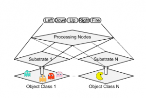
In “A Neuro-evolution Approach to General Atari Game Playing“, Hausknecht, Miikkulainen, and Stone (2013) describe and test four general game learning AIs based on evolving neural nets. They apply the AIs to sixty-one Atari 2600 games exceeding the best known human performance in three of the sixty-one games (Bowling, Kung Fu Master, and Video Pinball).  This work improves their previous Atari gaming AI described in “HyperNEAT-GGP: A HyperNEAT-based Atari General Game Player” (2012) with P. Khandelwal.

The Atari 2600 presents a uniform interface for all its games:  a 2D screen, a joystick, and one button.  The Atari 2600 games are simulated in the Arcade Learning Environment which has allowed several researchers to develop AIs for the Atari.

The four algorithms tested are:

  1. Fixed topology neural nets that adapt by changing weights between neurons
  2. Neural nets that evolve both the weights and the topology of the network (NEAT created by Stanley and Miikkulainen (2002))
  3. “Indirect encoding of the network weights”  (HyperNEAT created by Gauci and Stanley (2008)) 
  4. “A hybrid algorithm combining elements of both indirect encodings and individual weight evolution” (HybrID by Clune, Stanley, Pennock, and Ofria (2011))

All of the algorithms evolved a population of 100 individual neural nets over 150 generations mostly using the topology shown below.

nntopo

For MOVIES of the AIs in action click below

http://www.cs.utexas.edu/~mhauskn/projects/atari/movies.html


So I was thinking about how I should estimate the KL distance between two mixtures of Gaussians.  For discussion purposes, assume that the first mixture has pdf $f(x)$ and the second has pdf $g(x)$.

My fist thought was to randomly generate samples from $f(x)$ and to compute the average value of $\log(g(x))$ from the other mixture.  That would give me $E_f[\log(g(X))] = -H(f,g)$  and  $KL(f,g) = H(f,g) – H(f)$ where $H(f,g)$ is the cross entropy and $H(f)$ is the entropy.  This converges at order $1/\sqrt{n}$ and it is easy to program.

My second thought was to borrow an idea from Unscented Kalman filters.  I thought about creating a non-random sampling of from one distribution at specific points and estimating $E_f[\log(g(X))]$ from those points.

My third thought was to try Google.  Google suggested “Lower and Upper Bounds for Approximation of the Kullback-Leibler Divergence Between Gaussian Mixture Models” by Durrien, Thiran, and Kelly (2012) and “Approximating the Kullback Leibler divergence between Gaussian Mixture Models” by Hershey and Olsen (2007).  Here are some notes from their papers:

1.  The KL distance between two Gaussians $f$ and $g$ is

$D_{KL}( f || g ) = {1\over2}\left( \log\left( { \det(\Sigma_g)}\over { \det(\Sigma_f)}\right) + Tr( \Sigma_g^{-1}  \Sigma_f)  + ||\mu_f – \mu_g||_g^2 -d \right)$ where $d$ is the dimension of the space, $\Sigma$ is the covariance matrix, $\mu$ is the mean, $Tr$ is the trace, and

$|| x ||^2_g = x^T (\Sigma_g^{-1}) x$.

2.   Hershey and Olsen review several methods for estimating the divergence:

  • Monte-Carlo methods,  
  • Unscented methods (unscented methods are simple and an unscented approximation of $\int f(x) g(x) dx$ is exact if $f$ is a Gaussian and $g$ is quadratic),
  • Gaussian Approximation (this is bad, don’t do it, if you do do it, “I told you so”),
  • Product of Gaussian approximations using Jensen’s inequality (this is cute, I like it, but I’m not sure how accurate it is), and
  • Match Bound approximation by Do (2003) and Goldberg et al (2003) (just match each Gaussian with another Gaussian in the other mixture and compute those KL distances).

3.  Hershey and Olsen introduce a delightful improvement over Match Bound approximation using variational methods.  They have the same idea as Match Bound, but they significantly reduce the error in Jensen’s inequality by introducing weighted averages.  Since Jensen’s inequality produces a lower bound using the weighted average, they maximize the lower bound under all possible weightings. The maximizer happens to have a very simple form, so the bound is also is very simple to compute.  Very nice.  (Numerical results are given at the end of the paper.)  I’ve got to try this one out.

4.  Durrien, Thiran, and Kelly improve on the Hershey and Olsen method, but I’m not sure how much better the new method is.  More research required.