Languages

You are currently browsing the archive for the Languages category.

I’ve been reading “Category Theory for Programmers” which was suggested to me by Mark Ettinger.  This book presents many examples in C++ and Haskell.  It teaches you some Haskell as you read the book.  It uses almost zero upper level mathematics and it skips almost all of the mathematical formalities.  If you decide that you want to read it, then you might want to read the first six chapters of “Learn You a Haskell for Great Good!” and write a few small Haskell programs first.  (I also would suggest trying to solve the first three problems in Project Euler https://projecteuler.net/archives  using Haskell.)

I find the book to be easy to read and informative.  When the author makes a statement like   A*(B+C) = A*B + A*C where * means categorical product, + means coproduct, and = means isomorphic, I find myself trying to figure out the categories where the statement is true and the categories for which it is false.  (It is true for the Category of Set and the Category Hask.  The book is mostly about those categories.) That type of thinking improves my understanding of category theory.  The book is also reawakening the parts of my brain that had forgotten parts of category theory and Haskell.

Interestingly, in category theory, $A*(B+C) = A*B + A*C$ can be translated into the following theorems :

  1.  A*(B+C) = A*B + A*C  is true for all positive integers A,B, and C,
  2. max(A, min(B,C)) = min( max(A,B), max(A,C))  for all real numbers A, B, and C,
  3. lcm(A, gcd(B,C)) = gcd( lcm(A,B), lcm(A,C) )   where  lcm means least common multiple and gcd means greatest common denominator, and
  4. intersection(A, union(B,C)) = union( intersection(A,B), intersection(A, C)).
If you don’t believe the four theorems, here is some Mathematica Code which tests each theorem:
Unprotect[C];
test[ funcRandChoose_, prod_, sum_, i_] := Tally[ Table[ 
     A = funcRandChoose[];
     B = funcRandChoose[];
     C = funcRandChoose[];
      prod[ A, sum[B, C]] == sum[ prod[A, B] , prod[A, C]], 
 {i}]];

test[ RandomInteger[{1, 1000}] &, Times, Plus, 100]
test[ RandomInteger[{-1000, 1000}] &, Max, Min, 100]
test[ RandomInteger[{-1000, 1000}] &, LCM, GCD, 100]
test[ RandomSample[ Subsets[ Range[5]]] &, Intersection, Union, 100]
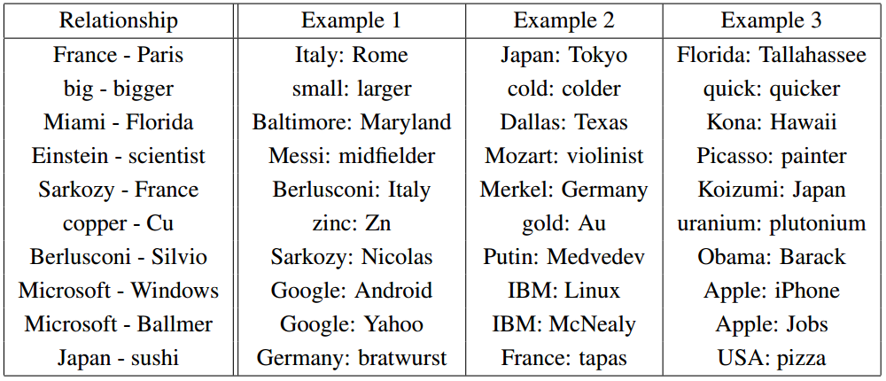
 

Christopher Olah wrote an incredibly insightful post on Deep Neural Nets (DNNs) titled “Deep Learning, NLP, and Representations“.  In his post, Chris looks at Deep Learning from a Natural Language Processing (NLP) point of view.  He discusses how many different deep neural nets designed for different NLP tasks learn the same things.   According to Chris and the many papers he cites, these DNNs will automatically learn to intelligently embed words into a vector space.  Words with related meanings will often be clustered together.  More surprisingly, analogies such as “France is to Paris as Italy is to Rome” or “Einstein is to scientist as Picasso is to Painter” are also learned by many DNNs when applied to NLP tasks.  Chris reproduced the chart of analogies below from “Efficient Estimation of Word Representations in Vector Space” by Mikolov, Chen, Corrado, and Dean (2013).

Relationship pairs in a word embedding. From Mikolov et al. (2013).

Additionally, the post details the implementation of recurrent deep neural nets for NLP.  Numerous papers are cited, but the writing is non-technical enough that anyone can gain insights into how DNNs work by reading Chris’s post.

So why don’t you just read it like NOW  — CLICK HERE.   :)


I’m quite excited by the Nuit Blanche post on the papers “Structure Discovery in Nonparametric Regression through Compositional Kernel Search” (Duvenaudy, Lloydy, Grossez, Tenenbaumz, Ghahramaniy 2013) and “Exploiting compositionality to explore a large space of model structures” (Grosse, Salakhutdinovm, Freeman, and Tenenbaum 2012).  For years my old company Momentum Investment Services, Carl, and I have been looking for fast, systematic ways to search large hypothesis spaces.  We considered context-free grammars as a means of generating hypothesis.  Carl and I did not get anywhere with that research, but now it seems that others have succeeded.  Be sure to look over the article, the blog posts, and the comments.

Check out

In the short, well written paper “An Estimate of an Upper Bound for the Entropy of English“, Brown, Stephan Della Pietra, Mercer, Vincent Della Pietra, and Lai (1992) give an estimated upper bound for English of 1.75 bits per character.  That estimate was somewhat lower than Shannon’s original upper bound of 2.3 bits per character. Along the way they give nice simple explanations of entropy and cross-entropy as applied to text.  More recently Montemurro and Zanette (2011) showed the entropy of all languages is around 3.5 bits per word. (see Wired Article and Plos One)

Julia can be written like Malab without typing information and it runs very fast, at nearly the speed of C, because it does runtime type inference and JIT compilation. Underneath it has sophisticated dynamic algebraic typing system which can be manipulated by the programmer (much like Haskell).  Carl sent me a link to this video about how the language achieves this level of type inference and type manipulation.

In “Semantic Hashing“, Salakhutdinov and Hinton (2007) show how to classify documents with binary vectors.  They combine deep learning and graphical models to assign each document a binary vector.  Similar documents can be found by using the L1 difference between the binary vectors.  Here is their abstract.

We show how to learn a deep graphical model of the word-count vectors obtained from a large set of documents. The values of the latent variables in the deepest layer are easy to infer and give a much better representation of each document than Latent Semantic Analysis. When the deepest layer is forced to use a small number of binary variables (e.g. 32), the graphical model performs “semantic hashing”: Documents are mapped to memory addresses in such away that semantically similar documents are located at nearby addresses. Documents similar to a query document can then be found by simply accessing all the addresses that differ by only a few bits from the address of the query document. This way of extending the efficiency of hash-coding to approximate matching is much faster than locality sensitive hashing, which is the fastest current method. By using semantic hashing to filter the documents given to TF-IDF, we achieve higher accuracy than applying TF-IDF to the entire document set.

The NLTK Python Library contains a large number of packages for text manipulation and classification.  It includes routines for classification (maximum entropy, naive Bayes, support vector machines, an interface to the Weka library, expectation maximization, k-means, conditional random fields,…), text-manipulation, parsing, and graphics.

About a year ago, I wrote a simple prime testing algorithm to test the speed of several languages.   I just added Julia (windows binary) to the list.

Time Language

0.3  Julia
0.3  VB 6.0 Compiled
0.3  VC++ 6.0
0.4  Digital Mars C
0.5  GHC Haskell Compiled with -O2 flag
0.7  Netbeans 6.9 Java
0.8  VB 6.0 (Interpreted strong typed)
1.3  Mathematica 8 compiled with Compilation Target->”C” 
1.9  Matlab 7.10.0.499 (R2010a)
2.5  GHC Haskell Compiled
3.6  “Compiled” Mathematica 8 
3.7  QiII SBC
5.0  Python IDLE 2.6.4
6    1992 Turbo C
7    Compiled PLT Scheme
7    VB 6.0 (Interpreted no type info)
7    Excel VBA (Iterp)
9    Clojure (Clojure Box 1.2 with type coersion)
11   "Compiled" Mathematica 7
19   PLT Scheme
20   netbeans python
20   ruby 1.8.6 for Windows
25   QiII Clisp
40   Emacs lisp using Cygwin
117  Mathematica 7
131  Mathematica 8
185  GHC Haskell Interactive Mode

Paper.js

Carl sent me this link.  Check it out.  Fun!


« Older entries