Reinforcement Learning

You are currently browsing the archive for the Reinforcement Learning category.

AlphaGo is changing how the Game is Played

May 18, 2017 in Deep Belief Networks, Games, General ML, Neural Nets, Reinforcement Learning by hundalhh | Permalink

In March of 2016, the computer program AlphaGo defeated Lee Sedol, one of the top 10 Go players in the world, in a five game match. Never before had a Go computer program beaten a professional Go player on the full size board. In January of 2017, AlphaGo won 60 consecutive online Go games against many of the best Go players in the world using the online pseudonym Master. During these games, AlphaGo (Master) played many non-traditional moves—moves that most professional Go players would have considered bad before AlphaGo appeared. These moves are changing the Go community as professional Go players adopt them into their play.

Michael Redmond, one of the highest ranked Go players in the world outside of Asia, reviews most of these games on You Tube. I have played Go maybe 10 times in my life, but for some reason, I enjoy watching these videos and seeing how AlphGo is changing the way Go is played. Here are some links to the videos by Redmond.

Two Randomly Selected Games from the series of 60 AlphaGo games played in January 2017

https://www.youtube.com/watch?v=gWabLAkvpIQ

https://www.youtube.com/watch?v=G5OKn2lWICk

Match 1 – Google DeepMind Challenge Match: Lee Sedol vs AlphaGo
https://www.youtube.com/watch?v=vFr3K2DORc8

The algorithms used by AlphaGo (Deep Learning, Monte Carlo Tree Search, and convolutional neural nets) are similar to the algorithms that I used at Penn State for autonomous vehicle path planning in a dynamic environment. These algorithms are not specific to Go. Deep Learning and Monte Carlo Tree Search can be used in any game. Google Deep Mind has had a lot of success applying these algorithms to Atari video games where the computer learns strategy through self play. Very similar algorithms created AlphaGo from self play and analysis of professional and amateur Go games.

I often wonder what we can learn about other board games from computers. We will learn more about Go from AlphaGo in two weeks. From May 23rd to 27th, AlphaGo will play against several top Go professionals at the “Future of Go Summit” conference.

Cheers,
Hein

Counterfactual Regret Minimization

April 11, 2017 in Games, General ML, Reinforcement Learning by hundalhh | Permalink

Gettysburg University has a nice webpage on Counterfactual Regret. Counterfactual Regret was used by the University of Alberta to solve the heads up limit Holdem poker game. (See e.g. the pokernews.com article).

Link: In Two Moves, AlphaGo and Lee Sedol Redefined the Future

March 16, 2016 in Games, Neural Nets, Reinforcement Learning by hundalhh | Permalink

Wired has a nice article about the two most brilliant moves in the historic match between AlphaGo and Lee Sedol.

http://www.wired.com/2016/03/two-moves-alphago-lee-sedol-redefined-future/

A Short Informal Description of Partially Observable Markov Decision Processes

May 3, 2015 in Reinforcement Learning by hundalhh | Permalink

A partially observable Markov decision process (POMDP) can be informally defined as a world in which an agent can take actions and gain rewards. The world has a set of possible world states S. This set can be finite (e.g. mine sweeper) or infinite (e. g. a robotic car in a parking lot). The world is only partially observable, so if we try to program an agent to act in this world, the robot does not know the state of the entire world, rather it only gets observations that partially reveal the state of the world. The set of possible observations is typically called Ω. The agent in a POMDP can take actions. The actions set is usually called A. The actions affect the world and result in rewards which also depend on the state of the world. (Technically, for every world state s and action a there is a reward R(s, a). R(s, a) is a real number. Also, for every world state s and action a there is a probability distribution of new possible world states that result after taking action a when the world is in state s.)

University of Alberta Solves Poker

January 9, 2015 in Games, General ML, Reinforcement Learning by hundalhh | Permalink

The Daily Mail reports that the Computer Poker Research Group at the University of Alberta seems to have solved heads-up limit hold’em poker.

You can play against their AI online.

(My thanks to Glen for emailing me the story!)

A review of “Playing Atari with Deep Reinforcement Learning”

December 10, 2014 in Games, General ML, Neural Nets, Reinforcement Learning by hundalhh | Permalink

Mnih, Kavukcuoglu, Silver, Graves, Antonoglon, Wierstra, and Riedmiller authored the paper “Playing Atari with Deep Reinforcement Learning” which describes and an Atari game playing program created by the company Deep Mind (recently acquired by Google). The AI did not just learn how to pay one game. It learned to play seven Atari games without game specific direction from the programmers. (The same learning parameters, neural network topologies, and algorithms were used for every game).

The 2600 Atari gaming system was quite popular in the late 1970’s and the early 1980’s. The games ran with only four kilobytes of RAM and a 210 x 160 pixel display with 128 colors. Various machine learning techniques have been applied to the old Atari games using the Arcade Learning Environment which precisely reproduces the Atari 2600 gaming system. (See e.g. “An Object-Oriented Representation for Efficient Reinforcement Learning” by Diuk, Cohen, and Littman 2008, ”HyperNEAT-GGP:A HyperNEAT-based Atari General Game Player” by Hausknecht, Khandelwal, Miikkulainen, and Stone 2012, “Application of TEXPLORE on Atari Games “ by Shung Zhang , ”A Neuroevolution Approach to General Atari Game Playing” by Hausknect, Lehman,” Miikkulalianen, and Stone 2014, and “Replicating the Paper ‘Playing Atari with Deep Reinforcement Learning’ ” by Korjus, Kuzovkin, Tampuu, and Pungas 2014.)

Various papers have been written on how computers can learn to pay the Atari games, but most of them used the abstract representations of objects on the screen within the emulator. The Mnih et al AI learned to play the games using only the raw 210 x 160 video and the score. It seems to be the first successful attempt to learn arcade gaming from raw video.

To learn from raw video, they first converted the video to grayscale and then downsampled/cropped to 84 x 84 images. The last four frames were used to determine actions. The 28224 input pixels were run through two hidden convolution neural net layers and one fully connected (no convolution) 256 node hidden layer with a single output for each possible action. Training was done with stochastic gradient decent using random samples drawn from a historical database of previous games played by the AI to improve convergence (This technique known as “experience replay” is described in “Reinforcement learning for robots using neural nets” Long-Ji Lin 1993.)

The objective function for supervised learning is usually a loss function representing the difference between the predicted label and the actual label. For these games the correct action is unknown, so reinforcement learning is used instead of supervised learning. The authors used a variant of Q-learning to train the weights in their neural network. They describe their algorithm in detail and compare it to several historical reinforcement algorithms, so this section of the paper can be used as a brief introduction to reinforcement learning.

The AI was trained to play seven games: Beam Rider, Breakout, Enduro, Pong, Q*bert, Seaquest, and Space Invaders. In six of the seven games, this general game learning algorithm outperformed all previously known reinforcement learning algorithms tested on those games and “surpasses a human expert on three” of the seven games.

An AI for 2048 — Part 1

March 17, 2014 in Games, Reinforcement Learning by hundalhh | Permalink

So I played the game 2048 and thought it would be fun to create an AI for the game. I wrote my code in Mathematica because it is a fun, terse language with easy access to numerical libraries since I was thinking some simple linear or logit regression ought to give me some easy to code strategies.

The game itself is pretty easy to code in Mathematica. The game is played on a 4×4 grid of tiles. Each tile in the grid can contain either a blank (I will hereafter use a _ to denote a blank), or one of the numbers 2,4,8,16,32,64,128, 256, 512, 1024, or 2048. On every turn, you can shift the board right, left, up, or down. When you shift the board, any adjacent matching numbers will combine.

The object of the game is to get one 2048 tile which usually requires around a thousand turns.

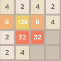
Here’s an example. Suppose you have the board below.

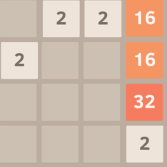
If you shift right, the top row will become _, _, 4, 16, because the two twos will combine. Nothing else will combine.

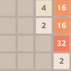
Shifting left gives the same result as shifting right except all of the tiles are on the left side instead of the right.

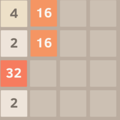
If we look back at the original image (below), we can see that there are two sixteen tiles stacked vertically.

So the original board (above) shifted down combines the two sixteens into a thirty-two (below) setting some possible follow-up moves like combining the twos on the bottom row or combining the two thirty-twos into a sixty-four.

There are a few other game features that make things more difficult. After every move, if the board changes, then a two or four tile randomly fills an empty space. So, the sum of the tiles increases by two or four every move.

Random Play

The first strategy I tried was random play. A typical random play board will look something like this after 50 moves.

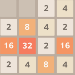
If you play for a while, you will think that this position is in a little difficult because the high numbers are not clumped, so they might be hard to combine. A typical random game ends in a position like this one.

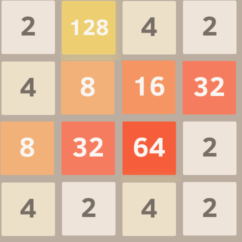
In the board above, the random player is in deep trouble. His large tiles are near the center, the 128 is not beside the 64, there are two 32 tiles separated by the 64, and the board is almost filled. The player can only move up or down. In this game the random player incorrectly moved up combining the two twos in the lower right and the new two tile appeared in the lower right corner square ending the game.

I ran a 1000 random games and found that the random player ends the game with an average tile total of 252. Here is a histogram of the resulting tile totals at the end of all 1000 games.

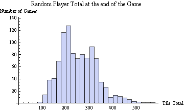
(The random player’s tile total was between 200 and 220 one hundred and twenty seven times. He was between 400 and 420 thirteen times.)

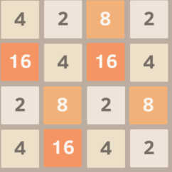
The random player’s largest tile was 256 5% of the time, 128 44% of the time, 64 42% of the time, 32 8% of the time, and 16 0.5% of the time. It seems almost impossible to have a max of 16 at the end. Here is how the random player achieved this ignominious result.

The Greedy Strategy

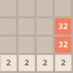
So what’s a simple improvement? About the simplest possible improvement is to try to score the most points every turn—the greedy strategy. You get the most points by making the largest tile possible. In the board below, the player has the options of going left or right combining the 32 tiles, or moving up or down combining the two 2 tiles in the lower left.

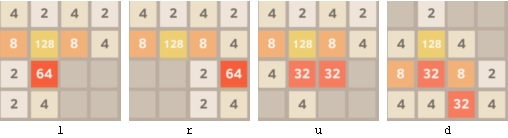
The greedy strategy would randomly choose between left or right combining the two 32 tiles. The greedy action avoids splitting the 32 tiles.

I ran 1000 greedy player games games. The average tile total at the end of a greedy player simulation was 399—almost a 60% improvement over random play. Here is a histogram of the greedy player’s results.

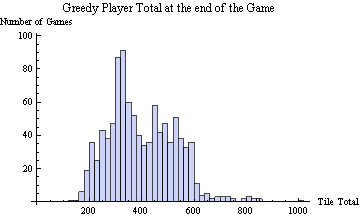
If you look closely, you will see that is a tiny bump just above 1000. In all 1000 games, the greedy player did manage to get a total above 1000 once, but never got the elusive 1024 tile. He got the 512 tile 2% of the time, the 256 tile 43% of the time, the 128 44%, the 64 11%, and in three games, his maximum tile was 32.

I ran a number of other simple strategies before moving onto the complex look ahead strategies like UCT. More on that in my next post.

“Generalized Thompson sampling for sequential decision-making and causal inference”

March 28, 2013 in Multi-Armed Bandit Problem, Reinforcement Learning by hundalhh | Permalink

In “Generalized Thompson sampling for sequential decision-making and causal inference“, Ortega and Braun (2013) give a short history of Thompson sampling (see [1], [2], [3], [4]) and report on the relationship between intelligent agents, evolutionary game theory, Bayesian inference, KL Divergence, and Thompson sampling. They develop a generalization of Thompson sampling based on a Bayesian prior over a distribution of environments. Some numerical results are provided. Here’s the abstract:

Recently, it has been shown how sampling actions from the predictive distribution over the optimal action—sometimes called Thompson sampling—can be applied to solve sequential adaptive control problems, when the optimal policy is known for each possible environment. The predictive distribution can then be constructed by a Bayesian superposition of the optimal policies weighted by their posterior probability that is updated by Bayesian inference and causal calculus. Here we discuss three important features of this approach. First, we discuss in how far such Thompson sampling can be regarded as a natural consequence of the Bayesian modeling of policy uncertainty. Second, we show how Thompson sampling can be used to study interactions between multiple adaptive agents, thus, opening up an avenue of game-theoretic analysis. Third, we show how Thompson sampling can be applied to infer causal relationships when interacting with an environment in a sequential fashion. In summary, our results suggest that Thompson sampling might not merely be a useful heuristic, but a principled method to address problems of adaptive sequential decision-making and causal inference.

Reinforcement Learning for Linear Control Systems

January 2, 2013 in Control Systems, Reinforcement Learning by hundalhh | Permalink

In “Efﬁcient Reinforcement Learning for High Dimensional Linear Quadratic Systems” Ibrahimi, Javanmard, and Van Roy (2012) present a fast reinforcement learning solution for linear control systems problems with quadratic costs. The problem is to minimize the total cost $\min_u \sum_{i=1}^T x_i^t Q x_i + u_i^t R u_i$ for the control system $x_{i+1} = A x_i + B u_i + w_i$ where $x\in R^j$ is the state of the system; $u\in R^k$ is the control; $Q, R, A,$ and $B$ are matrices; and $w_i\in R^j$ is a random multivariate normally distributed vector.

The 20 most striking papers, workshops, and presentations from NIPS 2012

December 18, 2012 in Deep Belief Networks, General ML, Graphical Models, Multi-Armed Bandit Problem, Neural Nets, Reinforcement Learning by hundalhh | Permalink

NIPS was pretty fantastic this year. There were a number of breakthroughs in the areas that interest me most: Markov Decision Processes, Game Theory, Multi-Armed Bandits, and Deep Belief Networks. Here is the list of papers, workshops, and presentations I found the most interesting or potentially useful:

Unfortunately, when you have 30 full day workshops in a two day period, you miss most of them. I could only attend the three listed above. There were many other great ones.

« Older entries

Artificial Intelligence Blog