Check out
“An introduction to Category Theory for Software Engineers” by Steve Easterbrook.
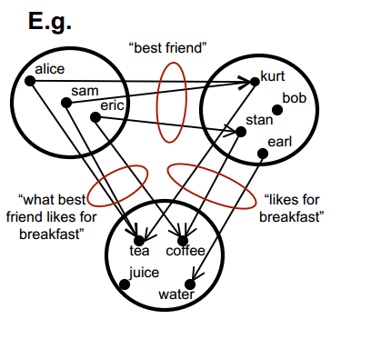
A category from “An introduction to Category Theory for Software Engineers” by Steve Easterbrook
We're blogging machines!
You are currently browsing the monthly archive for September 2013.
Check out
“An introduction to Category Theory for Software Engineers” by Steve Easterbrook.
A category from “An introduction to Category Theory for Software Engineers” by Steve Easterbrook
As I look at the hit statistics for the last quarter, I cannot help but wonder how well they fit Zipf’s law (a.k.a. Power Laws, Zipf–Mandelbrot law, discrete Pareto distribution). Zipf’s law states that the distribution of many ranked things like city populations, country populations, blog hits, word frequency distribution, probability distribution of questions for Alicebot, Wikipedia Hits, terrorist attacks, the response time of famous scientists, … look like a line when plotted on a log-log diagram. So here are the numbers for my blog hits and, below that, a plot of log(blog hits) vs log(rank) :
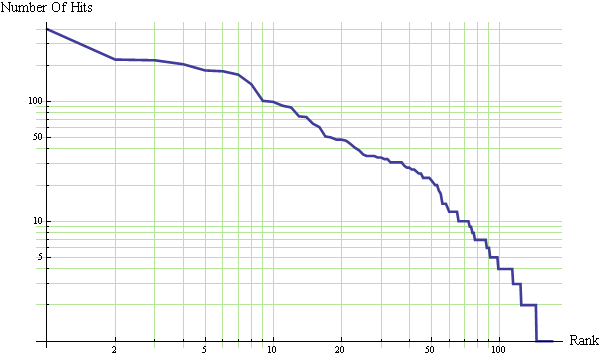
Not too linear. Hmmm.
(Though Zipf’s “law” has been known for a long time, this post is at least partly inspired by Tarence Tao’s wonderful post “Benford’s law, Zipf’s law, and the Pareto distribution“.)
So I have been reading a number of texts in my quest to learn category theory and apply it to AI. Two of the most interesting introductions to category theory are “Category Theory for Scientists” by Spivak (2013) and “Ologs: A Categorical Framework for Knowledge Representation” by Spivak and Kent (2012).
Ologs are a slightly more sophisticated, mathematical form of semantic networks.
Semantic networks are a graphical method for representing knowledge. Concepts are drawn as words (usually nouns) in boxes or ovals. Relationships between concepts are depicted as lines or arrows between concepts. (In graph theory, theses would be called edges.) Usually, the lines connecting concepts are labeled with words to describe the relationship. My favorite semantic network is the semantic network describing the book “Gödel Escher Bach“, but here is a simpler example.

A Semantic Network
Mathematically, semantic networks are a graph where the nodes are concepts and the edges are relationships. There are some cool algorithms for constructing semantic networks from text (see e.g. “Extracting Semantic Networks from Text via Relational Clustering” by Kok and Domingos (2008)).
Though semantic networks look like probabilistic graphical models (PGMs, a.k.a. Bayesian networks), they are different. In PGMs, the nodes are random variables not general classes and if five edges point to a node, then there is an associated five parameter, real-valued function associated with those five edges indicating the likelihood that the target variable has a particular value.
As I said before, Ologs are a more sophisticated directed graph. In Ologs, the nodes are typically nouns that can be assigned to one of many values. In directed graphs the edge starts at one node called the tail and ends at another node called the head. The edges in Ologs represent functions that given a value with the type of the tail node give you one value with the type of the head node. In the example shown below, the box “a date” could be assigned the values “Oct 12, 2010″ or “January 5, 2011″. The corresponding values of the “a year” would be 2010 and 2011.
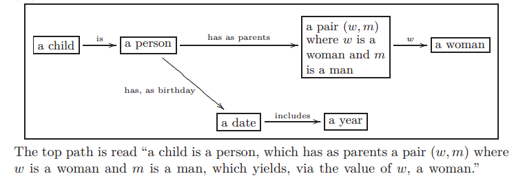
Example Olog from “Ologs: A categorical framework for knowledge representation”
In category theory, categories are directed graphs where the edges are called arrows and they have some specific properties. Ologs are part of the category Set. One of the important properties of arrows is that if the head of one arrow is the tail of another arrow, then a third arrow is implied which is called the composition of the original two arrows. In the diagram above the arrows “has, as birthday” and “includes” can be combined to create a new arrow from “a person” to “a year” which assigns to each person his or her birth year.
I just wanted to introduce categories and Ologs for later articles.
Cheers – Hein
Orthogonal functions are very useful and rather easy to use. The most famous ones are sin(n x) and cos(n x) on the interval [$-\pi$, $\pi$]. It is extremely easy to do linear regression with orthogonal functions.
Linear regression involves approximating a known function $f(x)$ as the weighted sum of other functions. This shows up all the time in various disguises in machine learning:
For orthogonal functions, computing the linear regression is simple. Suppose that the features are $f_1, f_2, \ldots, f_n$ and the functions $f_i$ are orthonormal, then the best approximation of the function $g(x)$ is the same as the solution to the linear regression
$$ g(x) \approx \sum_{i=1}^n \alpha_i f_i(x)$$
where $\alpha_i$ is the “inner product” of $f_i$ and $g$ denoted
$\alpha_i= \langle\;g, f_i\rangle = \int g(x) f(x) w(x) dx.$ (Two function are orthogonal if their inner product (or dot product) is zero. The set of orthogonal functions $\{f_i\}$ is called orthonormal if $<f_i, f_i>=1$ for all $i$.) The function $w(x)$ is a positive weight function which is typically just $w(x)=1$.
For example, if we try to approximate the function $g(x)=x^2$ on the interval [-1,1] by combining the features $f_1(x) = 1/\sqrt(2)$ and $f_2(x) = x \sqrt{3 \over 2} $, then
$$ g(x) \approx \sum_{i=1}^n \alpha_i f_i(x)$$
where
$$\alpha_1 = \langle g, f_1\rangle = \int_{-1}^1 g(x) f_1(x) dx = \int_{-1}^1 x^2 1/\sqrt2 dx = \sqrt{2}/3,$$
$$\alpha_2 = \langle g, f_2\rangle = \int_{-1}^1 g(x) f_2(x) dx= \int_{-1}^1 x^2 \sqrt{3/2}\; x dx =0,$$
and the best approximation is then $\sum_{i=1}^n \alpha_i f_i(x) = \alpha_1 f_1(x) = 1/3$.
The other day I needed to do a linear regression and I wanted to use orthogonal functions, so I started by using the trigonometric functions to approximate my function $g(x)$. Using trig functions to approximate another function on a closed interval like [-1,1] is the same as computing the Fourier Series. The resulting approximations were not good enough at x=-1 and x=1, so I wanted to change the weight function $w(x)$. Now assume that $u_1(x), u_2(x), \ldots, u_n(x)$ are orthonormal with the weight function w(x) on [-1,1]. Then
$$ \int_{-1}^1 u_i(x) u_j(x) w(x) dx = \delta_{i,j}$$
where $\delta_{i,j}$ is one if $i=j$ and zero otherwise. If we make a change of variable $x=y(t)$, then
$$ \int_{y^{-1}(-1)}^{y^{-1}(1)} u_i(y(t)) u_j(y(t)) w(y(t)) y'(t) dx = \delta_{i,j}.$$
It would be nice if
$$(1)\quad w(y(t)) y'(t)=1,$$
because then I could just set $u_i(y(t))$ equal to a trig function and the resulting $u_i(x)$ would be orthonormal with respect to the weight function $w(x)$. Condition (1) on $y$ is really an ordinary differential equation
$$y’ = {1\over{w(y)}}.$$
In order to get a better fit at $x=\pm 1$, I tried two weight functions $w(x) = {1\over{(1-x)(1+x)}}$ and $w(x) = {1\over{\sqrt{(1-x)(1+x)}}}$. For the former, the differential equation has solutions that look similar to the hyperbolic tangent function. The latter $w(x)$ yields the nice solution
$$y(t) = \sin( c + t).$$
So now if I choose $c=\pi/2$, then $y(t) = \cos(t)$, $y^{-1}(-1) = \pi$, $y^{-1}(1)=0$, so I need functions that are orthonormal on the interval $[-\pi, 0]$. The functions $\cos(n x)$ are orthogonal on that interval, but I need to divide by $\sqrt{\pi/2}$ to make them orthornormal. So, I set $u_n(y(t)) = \sqrt{2/\pi}\cos(n\;t)$ and now
$$ \int_{-1}^1 {{u_i(x) u_j(x)}\over {\sqrt{(1-x)(1+x)}}} dx = \delta_{i,j}.$$
The $u_n(x)$ functions are orthonormal with respect to the weight $w(x)$ which is exactly what I wanted.
Solving for $u(x)$ yields
$$u_n(x) = \sqrt{2/\pi} \cos( n \;\arccos(x)),$$
$$u_0(x) = \sqrt{2/\pi}, u_1(x) = \sqrt{2/\pi} x,$$
$$u_2(x) = \sqrt{2/\pi}(2x^2-1), u_3(x) = \sqrt{2/\pi}(4x^3-3x),\ldots.$$
If you happen to be an approximation theorist, you would probably notice that these are the Chebyshev polynomials multiplied by $\sqrt{2/\pi}$. I was rather surprised when I stumbled across them, but when I showed this to my friend Ludmil, he assured me that this accidental derivation was obvious. (But still fun ![]() )
)
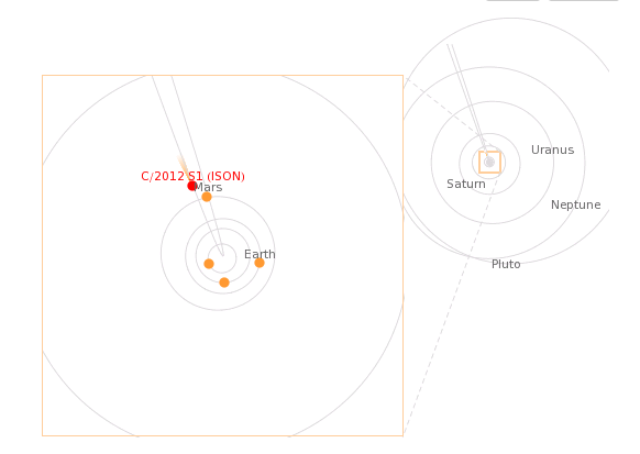
Comet ISON passing Mars
Comet Ison passing Mars (Wolfram Alpha)
I just got back from the Black Forest Star Party where Dr. Carey Lisse, head of NASA’s ISON Observing Campaign, gave a speech on comet ISON.
Comet ISON (see [1], [2]) is passing by Mars soon (Oct 1) and it will be “grazing the sun” before the end of the year, so I wondered if there was some relationship between the orbital period of a planet and the time it takes a passing comet to go from the planet to the Sun. Turns out there is a relationship. Here’s the approximate rule:
Time to sun $\approx$ Orbital Period / $ 3 \pi \sqrt{2} \approx $ Orbital Period / 13.3 !
In the case of ISON and Mars,
Time to sun $\approx$ 687 days / 13.3 $\approx$ 52 days.
But Oct 1 + 52 days is Nov 22, and perihelion is on Nov 28. Why so far off?
Well, turns out that Mars is farther from the sun than usual. If we correct for that, then the formula estimates perihelion to within 1 day—much better.
For those that like derivations, here is the derivation for the 13.3 rule.
The orbital period of a planet is $T_p = 2 \pi \sqrt{ r^3 \over {G m_S} }$ where $m_S$ is the mass of the Sun, $r$ is the radius of the planet’s orbit (or, more precisely, the semi-major axis of its orbit), and G = 6.67e-11 is the gravitational constant.
The speed of a comet from the Oort cloud is derived from its energy.
Kinetic Energy = -Potential Energy
$ \frac12 m v^2 = G m m_S / r$
$v = \sqrt{ {2 G m_S}\over{r}} $
where $r$ is the distance from the comet to the sun.
So the time for a Sun grazer to go from distance $r_0$ to the sun is about
$$T_S = \int_0^{r_0} {1\over v} dr $$
$$ = \int_0^{r_0} \sqrt{ r\over{2 G m_S}} dr $$
$$ = \frac13 \sqrt{ 2 r^3 \over{G m_S} }.$$
Finally,
$$T_p/T_S = {{2 \pi \sqrt{ r^3 \over {G m_S} }}\over{ \frac13 \sqrt{ 2 r^3 \over{G m_S} }}} = 3 \pi \sqrt{2} \approx 13.3.$$