Logic

You are currently browsing the archive for the Logic category.

Suppose that you are playing the game Minesweeper.  On your first move, you click on the lower left corner square and reveal a 1.  Then you click on the square above the corner and reveal a 2.  Then you click on the square above that and reveal a 3.  What is the “safest” next move?

Screen Shot 2021-02-08 at 9.31.51 AM

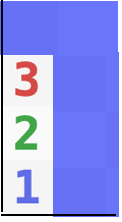
In order to talk about the contents of the blue squares, we will label them A,B,C,D, and E.

Screen Shot 2021-02-08 at 9.35.35 AM

There are only three possible scenarios:

a) A, B, C, and E have mines,

b) A, C, and D have mines, or

c) B, C, and D have mines.

But, not all of these scenarios are equally likely.  Suppose there are a total of $m$ mines on the board and $s$ squares left excluding the eight that we are looking at. Then the total number of possible distributions of the mines for scenarios a, b, and c are:

  • $n_a = {s\choose m-4},$
  • $n_b= {s\choose m-3},$ and
  • $n_c ={s\choose m-3}.$

These scenarios are not equally likely.  (Above we used choose notation.  ${n\choose m}= \frac{n!}{m! (n-m)!}$ where $n!=1\cdot2\cdot3\cdot\cdots\cdot n$.  For example 4!=24 and ${5\choose 2}=\frac{5!}{2!\  \cdot\ 3!} = \frac{120}{2 \cdot 6}= 10$.)  In fact,

$$\begin{aligned} r=\frac{n_b}{n_a}&=\frac{s\choose m-3}{s\choose m-4} \\&=\frac{\frac{s!}{(m-3)! (s-(m-3))!}}{\frac{s!}{(m-4)! (s-(m-4))!}}\\&=\frac{\frac{1}{(m-3)! (s-(m-3))!}}{\frac{1}{(m-4)! (s-(m-4))!}}\\&= \frac{(m-4)! (s-(m-4))!}{(m-3)! (s-(m-3))!}\\&= \frac{ (s-m+4)!}{(m-3) (s-m+3))!}\\&= \frac{ s-m+4}{m-3 }.\end{aligned}$$

In the beginning of the game $r\approx s/m-1\approx 4$, so scenarios b and c are about four times as likely as scenario a.  We can now estimate the probabilities of scenarios a, b, and c to be about

  • “probability of scenario a” = $p_a \approx 1/9,$
  • “probability of scenario b” = $p_b \approx 4/9, and$
  • “probability of scenario c” = $p_c \approx 4/9.$

We can now conclude that the probability that square A has a mine is 5/9, that square B has a mine is 5/9, that square C has a mine is 100%, that square D has a mine is 8/9, and that square E has a mine is 1/9, so square E is the “safest” move.

Generally speaking, scenarios with more mines are less likely if less than half of the unknown squares have mines.

Another interesting way to think about it is that the 3 and 2 squares pulled the mines toward them making square E less likely to contain a mine.

You can approximate the probability of each scenario by just assuming that the squares are independent random variables (a false, but almost true assumption) each of which has probability $m/s$ of containing a mine.  Using that method gives the same results as the approximation above.

If you prefer an exact calculation, then use the formula

$$ r=\frac{ s-m+4}{m-3 }$$

to get the exact ratio of $\frac{p_b}{p_a} = \frac{p_c}{p_a}=r$.


(PS:  Jennifer told me via email that you can play Minesweeper online at https://www.solitaireparadise.com/games_list/minesweeper.htm)


Hey, I just enrolled in Stanford’s General Game Playing CourseGeneral game playing programs are programs that try to play almost any game after being given the rules.  There is a yearly competition of general game playing programs at the AAAI conference.  If you join the course, send me an email so that we can exchange ideas or notes.  (my email address is hundal followed by “hh” at yahoo.com)

Cheers, Hein


Garvesh Raskutti has some nice slides on Probabilistic Graphical Models and Markov Logic Networks (Richardson & Domingos 2006).  Markov Logic Networks encode first order predicate logic into a Markov Random Field. The resulting networks can be quite large because statements like “for all x, y, and z, x is y’s parent and z is x’s parent imply z is y’s grandparent” require the existence of $2n^2$ nodes in the graph where $n$ is the number of people considered.  The resulting networks are frequently solved by using Gibbs Sampling.  For even more information Pedro Domingos has put an entire course online at

www.cs.washington.edu/homes/pedrod/803


Lifted Inference uses the rules of first order predicate logic to improve the speed of the standard Markov Random Field algorithms applied to Markov Logic Networks.  I wish I had been in Barcelona Spain in July last year for IJCAI11 because they had a cool tutorial on Lifted Inference.  Here’s a quote

Much has been achieved in the field of AI, yet much remains to be done if we are to reach the goals we all imagine. One of the key challenges with moving ahead is closing the gap between logical and statistical AI. Recent years have seen an explosion of successes in combining probability and (subsets of) first-order logic respectively programming languages and databases in several subfields of AI: Reasoning, Learning, Knowledge Representation, Planning, Databases, NLP, Robotics, Vision, etc. Nowadays, we can learn probabilistic relational models automatically from millions of inter-related objects. We can generate optimal plans and learn to act optimally in uncertain environments involving millions of objects and relations among them. Exploiting shared factors can speed up message-passing algorithms for relational inference but also for classical propositional inference such as solving SAT problems. We can even perform exact lifted probabilistic inference avoiding explicit state enumeration by manipulating first-order state representations directly.

In the related paper “Lifted Inference Seen from the Other Side : The Tractable Features“, Jha, Gogate, Meliou, Suciu (2010) reverse this notion.  Here’s the abstract:

Lifted Inference algorithms for representations that combine first-order logic and graphical models have been the focus of much recent research. All lifted algorithms developed to date are based on the same underlying idea: take a standard probabilistic inference algorithm (e.g., variable elimination, belief propagation etc.) and improve its efficiency by exploiting repeated structure in the first-order model. In this paper, we propose an approach from the other side in that we use techniques from logic for probabilistic inference. In particular, we define a set of rules that look only at the logical representation to identify models for which exact efficient inference is possible. Our rules yield new tractable classes that could not be solved efficiently by any of the existing techniques.

Answer:  Statistical Relational Learning.  Maybe I can get the book for Christmas.

The other day, Carl mentioned that Euclidean Geometry was decidable.  I thought that was impossible because I thought it would have an isomorphic copy of Peano arithmetic which is not decidable.   Later he pointed me toward Tarski’s axioms.   Here’s a quote from the Wikipedia page “This fact allowed Tarski to prove that Euclidean geometry is decidable: there exists an algorithm which can determine the truth or falsity of any sentence.”  I found the whole article to be pretty cool because I had never really dug into geometry as a first order predicate calculus.

Venn Diagrams

Carl sent me a link to a Venn diagrams post, so that got me thinking. A Venn Diagram with $n$ atoms has to represent $2^n$ regions. For example if $n$ is $2$, then you have the standard Venn diagram below.

Each time you increase $n$ by one, you double the number of regions.  This makes me think of binary codes and orthogonal functions. Everybody’s favorite orthogonal functions are the trig functions, so you should be able to draw Venn diagrams with wavy trig functions. Here was my first try.

Those seemed kind of busy, so I dampened the amplitude on the high frequencies (making the slopes that same and possibly increasing artistic appeal.)

I really like the last one.