May 2023

You are currently browsing the monthly archive for May 2023.

In Part 1, we defined the Second Banker’s problem and gave a formula for the optimal time to make a purchase.  All of the proofs are given in this PDF.


Interest Income immediately before the optimal purchase time for the Second Panker’s problem

As with the first banker’s problem, the income from interest just before the optimal purchase time is
$$
\mathrm{interest\ income\ during\ purchase} = \frac{c \;r_1 r_2 }{r_2-r_1}.
$$

Notice that this income does not depend on the initial amount in the bank account $B_0$.

For example, if

  • you initially have \$1000 in the account,
  • the cost of increasing the interest rate is \$1,100,
  • $r_1=0.05=5\%$, and
  • $r_2=0.08=8\%$,

then $$\begin{aligned}\mathrm{interest\ income\ during\ purchase} &= \frac{c \;r_1 r_2 }{r_2-r_1}\\&= \frac{ \$1100\cdot 0.05 \cdot 0.08}{0.08-0.05}\\&= \frac{ \$55 \cdot 0.08}{0.03} \approx \$146.67\mathrm{\ per\ year.}\end{aligned}$$

REMARK

Note that the interest income can also be expressed by
\begin{equation}
\label{eqone}
\mathrm{interest\ income\ during\ purchase} = c/t_{\mathrm{pay}}
\end{equation}
where
\begin{equation}
\label{eqtwo}
t_\mathrm{pay} = \frac1{r_1} – \frac1{r_2}= \frac{c}{B_0 r_1 \exp(r_1 t_\mathrm{buy})}
\end{equation}
is the amount of time it takes to pay $c$ dollars from interest starting at the optimal time $t_\mathrm{buy}$.

For the previous example, we get
$$
t_\mathrm{pay} = \frac1{r_1} – \frac1{r_2} = \frac1{0.05} – \frac1{0.08} = 20 – 12.5 = 7.5\mathrm{\ years,\ and}
$$
$$
\mathrm{interest\ income\ during\ purchase} = c/t_{\mathrm{pay}}= 1100/7.5 \approx \$146.67/\mathrm{year}.
$$


Recovery Time

If you do purchase the interest rate hike at the optimal time, how many years will you need to wait until the optimal strategy surpasses the never buy strategy. The recovery time for the second banker’s problem is almost, but not quite the same as the first banker’s problem. For the second banker’s problem,
$$
t_{\mathrm{surpass}} = t_{buy} + 1/r_1.
$$
For the example,
$$
t_{\mathrm{surpass}} \approx 21.5228+ \frac{1}{0.05} = 41.5228.
$$

SecRecover

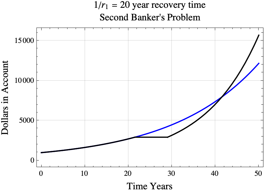
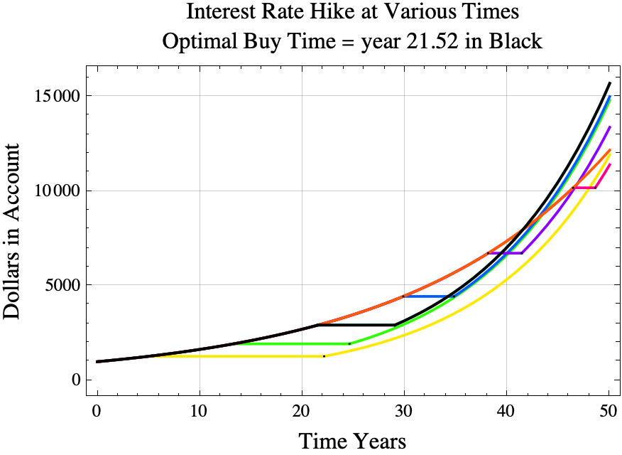
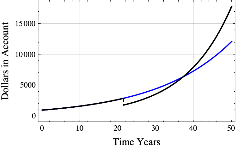
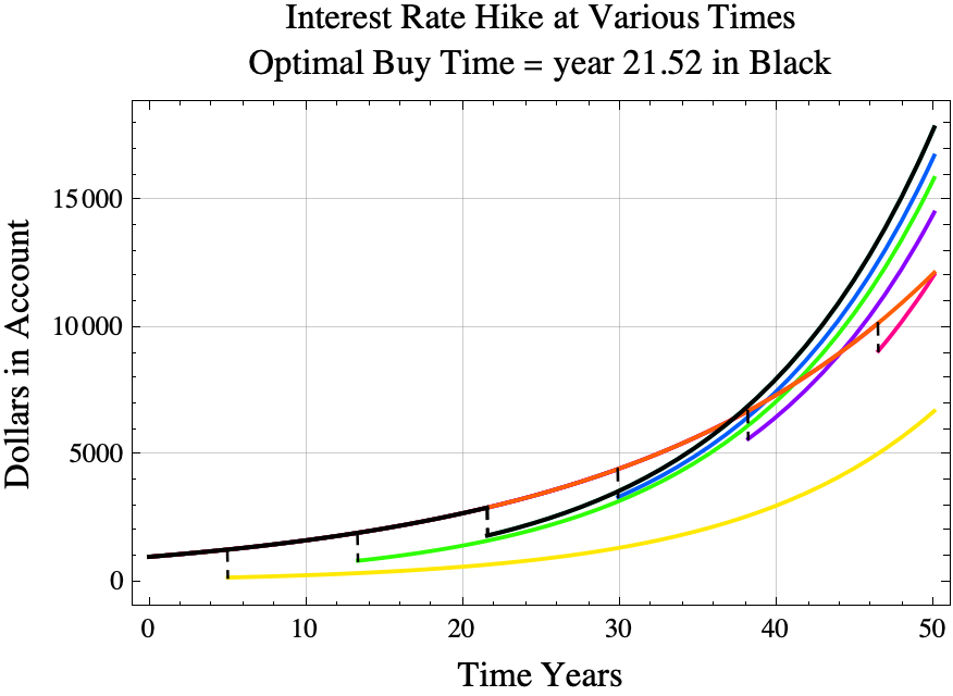
The black line shows the results of buying the interest rate increase at the optimal time. The blue line shows what happens if you never buy the interest rate hike and just continue to get 5% interest.
If you buy the interest rate hike at the optimal time, then you will maximize the account balance at all times $t>1/r_1$ years later. (Mathematically, for every $t> t_{\mathrm{buy}} + 1/r_1$, the strategy of purchasing the interest rate upgrade at time $t_{\mathrm{buy}}$ results in an account balance at time $t$ that exceeds the account balance at time $t$ using any other strategy.)

Consider the following game. You have a bank account that is compounded continuously with an interest rate of $r_1$. Your banker offers you the following deal. At any time in the future, you can pay $c$ dollars using only the interest from the account to increase your interest rate to $r_2$. If your balance is $b$ at the time of the upgrade, then your balance will remain at $b$ for $c/(r_1 b)$ years which is the time required to pay $c$ dollars from interest alone.  Other than paying for the interest upgrade, you can never add or subtract any money until retirement which is very far in the future. When should you accept the banker’s offer? Let’s call this game “the second banker’s problem”. (We assume that $c, r_1,$ and $r_2$ are positive real numbers and $1>r_2> r_1>0$.)

(This game is similar to purchasing a growth technology in the game Master of Orion (Original 1993 version).  For example, if you buy the “Improved Industrial Tech 9″ technology early in the game, the cost of factories is reduced for the remainder of the game. Reducing the cost of factories increases your economy’s growth rate.)

(All proofs for the second banker’s problem can be found in this PDF.)

 
For the first banker’s problem, the balance in the account is immediately reduced by $c$ dollars and the interest rate is immediately increased to $r_2$. See this blog post or this PDF for an analysis of the first banker’s problem. The third banker’s problem allows the saver to buy two separate interest rate increases.

 
For the second banker’s problem, you might be tempted to say that you should buy the interest rate increase as early as possible, but that might be bad if $c/(r_1 b)$ is a large number of years.  On the other hand, there is no reason to buy the interest rate upgrade if the time to retirement is less than $c/(r_1 b)$ years.

Optimal Purchase Time

Perhaps surprisingly, the optimal time to purchase the interest rate hike is the same for the first and the second banker’s problems. For either problem, you should take the deal at time
$$t_{\mathrm{buy}}=\frac{1}{r_1}\ln\left(\frac{c \; r_2 }{B_0(r_2-r_1)}\right)$$
where $B_0$ is the amount of money in the account at time zero, and $\ln(x)$ is the natural log. $$\ln(x) = \frac{\log_{10}(x)}{\log_{10}(e)}.$$ I was a bit surprised to find that the optimal purchase time $t_{\mathrm{buy}}$ for the second banker’s problem is the same as the optimal purchase time for the first banker’s problem.

The amount of money in the account at the optimal purchase time is $$b_{\mathrm{opt}} = \frac{c \; r_2 }{r_2-r_1}.$$

Example

For example, if

  • you initially have \$1000 in the account,
  • the cost of increasing the interest rate is \$1,100,
  • $r_1=0.05=5\%$, and
  • $r_2=0.08=8\%$,

then the the correct time to buy the interest rate increase is
$$
\begin{aligned}
t_{\mathrm{buy}}&=\frac{1}{r_1}\ln\left(\frac{c \; r_2 }{B_0(r_2-r_1)}\right)\\
&=\frac{1}{0.05}\ln\left(\frac{1100\cdot 0.08 }{1000(0.08-0.05)}\right)\\
&=\frac{1}{0.05}\ln\left(\frac{88 }{1000(0.03)}\right)\\
&=20\ln\left(\frac{88 }{30}\right)\\
&\approx21.5228\ \mathrm{years.}
\end{aligned}
$$

SecondBanker

SecondBLegend


In the diagram above, the black line shows the results of paying \$1,100 from interest starting at year 21.5228, the optimal time to start paying for the interest rate upgrade. The orange line shows what happens if the player does not invest before year 50. The yellow line shows the result if she or he starts paying for the investment on year 5.

In part 1, we described the “first banker’s problem” where you can pay a banker to increase your interest rate from $r_1$ to $r_2$ by removing $c$ dollars from your account.  The optimal time to purchase the rate increase is when you have

\begin{equation}
\mathrm{balanceBefore} =\frac{c \; r_2 }{r_2-r_1}
\end{equation}

dollars in your account.  (All of the formulas and theorems about the first banker’s problem as well as Python simulation code for the first banker’s problem and proofs can be found in this PDF.)


Interest Income immediately before the optimal purchase time

When compounding continuously, the amount of interest that you are earning at any time is the balance at that time times $r_1$.  The amount of interest income just before the optimal purchase time is

$$\mathrm{interst\ income\ immediately\ before\ purchase} = r_1\cdot \mathrm{balanceBefore} = \;\frac{r_1 r_2  c}{r_2-r_1}.$$

example

If

  • you initially have \$1000 in the account,
  • the cost of increasing the interest rate is \$1,100,
  • $r_1=0.05=5\%$, and
  • $r_2=0.08=8\%$,

then
$$
\begin{aligned}
\mathrm{income\ immediately\ before\ purchase} &= \frac{c \;r_1 r_2 }{r_2-r_1}\\
&= \frac{ \$1100\cdot 0.05 \cdot 0.08}{0.08-0.05}\\
&= \frac{ \$55 \cdot 0.08}{0.03} \approx \$146.67\mathrm{\ per\ year.}
\end{aligned}
$$

Recovery Time

If you do purchase the interest rate hike at the optimal time, how many years will you need to wait until the optimal strategy surpasses the never buy strategy? The answer is you will have to wait approximately $1/m$ years after the purchase where $m$ is the average of $r_1$ and $r_2$.  The exact time when the optimal strategy surpasses the never buy strategy is

$$
t_{\mathrm{surpass}} = t_{buy} + \frac{ \ln(r_2) – \ln(r_1)}{r_2-r_1}.
$$where $$t_{\mathrm{buy}}=\frac{1}{r_1}\ln\left(\frac{c \; r_2 }{B_0(r_2-r_1)}\right)$$

and $B_0$ is the amount in the account at time 0.  (Bounds for the expression $(\ln(r_2) – \ln(r_1) )/ (r_2 – r_1)$ can be found here.)

For the previous example,

$$t_{\mathrm{surpass}} \approx 21.5228+ \frac{ \ln(0.08) – \ln(0.05)}{0.08-0.05} \approx 37.1868.$$

BSurp

The black line shows the results of buying the interest rate at the optimal time. The blue line shows what happens if you never buy the interest rate hike and just continue to get 5% interest.

The number of years needed to catch up is between $1/r_2$ years and $1/r_1$ years. GPT wrote a nice proof of this fact.

If you buy the interest rate hike at the optimal time, then you will maximize the account balance at all times $t>1/r_1$ years later. (Mathematically, for every $t> t_{\mathrm{buy}} + 1/r_1$, the strategy of purchasing the interest rate upgrade at time $t_{\mathrm{buy}}$ results in an account balance at time $t$ that exceeds the account balance at time $t$ using any other strategy.

In the game Master of Orion and some related games, it is possible to purchase technologies that increase the rate of growth of your empire.  I wanted to simplify this idea enough to get clean mathematical solutions.  I call the resulting three simplified games the first, second, and third banker’s problems.

  1. In the first banker’s problem, the saver is offered a deal where they can buy an interest rate upgrade for a fixed amount of money paid from the account balance at any time specified by the saver.
  2. The second banker’s problem is the same as the first, except that the payment for the interest upgrade comes solely from account interest.
  3. For the third banker’s problem the saver can, at any time, upgrade from interest rate $r_1$ to interest rate $r_2$ for $c_1$ dollars and upgrade from $r_2$ to $r_3$ for $c_2$ dollars, or upgrade directly from interest rate $r_1$ to interest rate $r_3$ for $c_2$ dollars where $r_1<r_2<r_3$ and $c_1<c_2$.

This post will state the formula for computing the optimal time to buy the interest rate upgrade for the first banker’s problem, compute the optimal time to buy for one example, and show the results of buying at non-optimal times.

All of the formulas and theorems about the first banker’s problem as well as Python simulation code for the first banker’s problem and proofs can be found in this PDF.


the first banker’s problem

Consider the following game. You have a bank account that is compounded continuously with an interest rate of $r_1$. Your banker offers you the following deal. At any time in the future, if your account balance is greater than $c$ dollars, you can pay $c$ dollars from the account to increase your interest rate to $r_2$. You can only use the funds in the account to pay for this interest rate increase and you can never add or subtract any money until retirement which is very far in the future. When should you accept the banker’s offer?  (We assume that $c, r_1,$ and $r_2$ are positive real numbers and $1>r_2> r_1>0$.)

At first you might be tempted to say that you should buy the interest rate increase as early as possible, but it turns out that that is a bad idea. If you have exactly $c$ dollars in the account and you buy the rate increase, then you will have zero dollars in the account and you are stuck with zero dollars in the account until you retire. Similarly, if you have $c+\$0.01$ in the account and you buy the interest rate increase, then you will only have one cent in the account after the purchase, and it will take a long time to grow that one cent into a large amount of money.

On the other hand, it is probably wrong to wait until the last microsecond before you retire to buy an interest rate increase because the increased amount of interest that you receive is unlikely to be larger than the cost $c$.

The answer to the first banker’s problem is that you should take the deal at time

\begin{equation}
t_{\mathrm{buy}}=\frac{1}{r_1}\ln\left(\frac{c \; r_2 }{B_0(r_2-r_1)}\right)
\end{equation}
where $B_0$ is the amount of money in the account at time zero, and $\ln(x)$ is the natural log. $$\ln(x) = \frac{\log_{10}(x)}{\log_{10}(e)}.$$

At that time the balance before the purchase will be

\begin{equation}
\mathrm{balanceBefore} =\frac{c \; r_2 }{r_2-r_1},
\end{equation}

and the balance immediately after purchasing the interest upgrade will be

\begin{equation}
\mathrm{balanceAfter} =\frac{c \; r_1 }{r_2-r_1}.
\end{equation}


Example

For example, if

  • you initially have \$1000 in the account,
  • the cost of increasing the interest rate is \$1,100,
  • $r_1=0.05=5\%$, and
  • $r_2=0.08=8\%$,

then the the correct time to buy the interest rate increase is

$$
\begin{aligned}
t_{\mathrm{buy}}&=\frac{1}{r_1}\ln\left(\frac{c \; r_2 }{B_0(r_2-r_1)}\right)\\
&=\frac{1}{0.05}\ln\left(\frac{1100\cdot 0.08 }{1000(0.08-0.05)}\right)\\
&=\frac{1}{0.05}\ln\left(\frac{88 }{1000(0.03)}\right)\\
&=20\ln\left(\frac{88 }{30}\right)\\
&\approx21.5228\ \mathrm{years}
\end{aligned}
$$and the account balance before making the payment at the optimal time would be

$$\begin{aligned}\mathrm{balanceBefore} &=\frac{c \; r_2 }{r_2-r_1}\\&=\frac{1100 \cdot 0.08 }{0.08-0.05}\\&=\frac{88 }{0.03}\\&\approx \$2933.33.\end{aligned}$$

The diagram below shows what happens if you buy the interest upgrade at various times.  The purchases are represented as a black vertical dashed lines. The solid black line shows the results of paying \$1,100 at year 21.5228, the optimal time to invest. The red line shows what happens if the player does not invest before year 50. The yellow line shows the result if she or he invests on year 5.


Banker BLegend