Clustering

You are currently browsing the archive for the Clustering category.


Christopher Olah wrote an incredibly insightful post on Deep Neural Nets (DNNs) titled “Deep Learning, NLP, and Representations“.  In his post, Chris looks at Deep Learning from a Natural Language Processing (NLP) point of view.  He discusses how many different deep neural nets designed for different NLP tasks learn the same things.   According to Chris and the many papers he cites, these DNNs will automatically learn to intelligently embed words into a vector space.  Words with related meanings will often be clustered together.  More surprisingly, analogies such as “France is to Paris as Italy is to Rome” or “Einstein is to scientist as Picasso is to Painter” are also learned by many DNNs when applied to NLP tasks.  Chris reproduced the chart of analogies below from “Efficient Estimation of Word Representations in Vector Space” by Mikolov, Chen, Corrado, and Dean (2013).

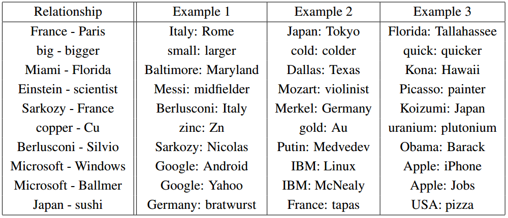
Relationship pairs in a word embedding. From Mikolov et al. (2013).

Additionally, the post details the implementation of recurrent deep neural nets for NLP.  Numerous papers are cited, but the writing is non-technical enough that anyone can gain insights into how DNNs work by reading Chris’s post.

So why don’t you just read it like NOW  — CLICK HERE.   :)


The Johnson–Lindenstrauss lemma roughly states that if you have large number of points in a high dimensional space, you can find a mapping to a lower dimensional space that almost preserves the distances between points. This lemma is useful for compressive sensingself-organizing maps (Kohonen maps) and manifold learning.  The following corollary is an immediate consequence of the lemma.

Corollary: For any positive integers $j>k$ and any set $S$ of $n$ points in $R^j$ there exists a mapping $f: R^j \rightarrow R^k$ such that for any two points $x,y \in S$,

$$(1 – \epsilon) ||x-y|| < ||f(x) – f(y)|| < (1 +\epsilon) ||x-y||$$

where

$$\epsilon = \sqrt{ 8 \log n \over k }.$$

According to the Wikipedia “The map used for the embedding is at least Lipschitz, and can even be taken to be an orthogonal projection.”

Ailon and Chazelle published an interesting approximate nearest neighbor algorithm based on “the Fast Johnson-Lindenstrauss Transform”.  They write “The FJLT is faster than standard random projections and just as easy to implement. It is based upon the preconditioning of a sparse projection matrix with a randomized Fourier transform.” and

By the Johnson-Lindenstrauss lemma [25,27,31], $n$ points in Euclidean space can be projected down to $k = O(\epsilon^{−2} \log n)$ dimensions while incurring a distortion of at most $1 + \epsilon$ in their pairwise distances. To achieve this requires a dense $k$-by-$d$ matrix; and so mapping each point takes $O(d \log n)$ time (for fixed $\epsilon$). Is that optimal? A lower bound of Alon [3] dashes any hope of reducing the number of rows (as a function of n), so the obvious question is whether the matrix can be made sparse.  Achlioptas [1] has shown that the density can be reduced by a constant factor, but one cannot go much further because a sparse matrix will typically distort a sparse vector. To prevent this, we use a central concept from harmonic analysis known as the Heisenberg principle (so named because it is the key idea behind the Uncertainty Principle): A signal and its spectrum cannot be both concentrated. With this in mind, we precondition the random projection with a Fourier transform (via an FFT) in order to isometrically enlarge the support of any sparse vector. To prevent the inverse effect, ie, the sparsification of dense vectors, we randomize the Fourier transform.


In “Autoencoders, MDL, and Helmholtz Free Energy“, Hinton and Zemel (2001) use Minimum Description Length as an objective function for formulating generative and recognition weights for an autoencoding neural net.  They develop a stochastic Vector Quantization method very similar to mixture of Gaussians where each input vector is encoded with

$$E_i = – \log \pi_i  – k \log t + {k\over2} \log 2 \pi \sigma^2 + {{d^2} \over{2\sigma^2}}$$

nats (1 nat = 1/log(2) bits = 1.44 bits) where $t$ is the quantization width, $d$ is the Mahalanobis distance to the mean of the Gaussian, $k$ is the dimension of the input space, $\pi_i$ is the weight of the $i$th Gaussian.  They call this the “energy” of the code.  Encoding only using this scheme wastes bits because, for example, there may be vectors that are equally distant from two Gaussian. The amount wasted is

$$H = -\sum p_i \log p_i$$

where $p_i$ the probability that the code will be assigned to the $i$th Gaussian. So the “true” expected description length is

$$F = \sum_i p_i E_i – H$$

which “has exactly the form of the Helmholtz free energy.”  This free energy is minimized by setting

$$p_i = {{e^{-E_i}}\over{\sum_j e^{-E_j}}}.$$

In order to make computation practical, they recommend using a suboptimal distributions “as a Lyapunov function for learning” (see Neal and Hinton 1993). They apply their method to learn factorial codes.


The blog Computational Information Geometry Wonderland pointed me toward the article “k-MLE: A fast algorithm for learning statistical mixture models” by Frank Nielsen (2012).  $k$-means can be viewed as alternating between 1) assigning points to clusters and 2) performing a maximum likelihood estimation (MLE) of the mean of spherical Gaussians clusters (all of which are forced to have the same covariance matrix equal to a scalar multiple of the identity).  If we replace the spherical Gaussian with another set of distributions, we get $k$-MLE.  Nielsen does a remarkably good job of introducing the reader to some complex concepts without requiring anything other than a background in probability and advance calculus.  He explores the relationships between $k$-MLE with exponential families and information geometry.  Along the way he exposes the reader to Bregman divergences,  cross-entropy,  Legendre dualityItakura-Saito divergence, and Burg matrix divergence.

In “Clustering via Dirichlet Process Mixture Models for Portable Skill Discovery“, Niekum and Barto (2011) apply Sub-goal Discovery and Skill Discovery to improve Reinforcement Learning on Markov Decision Processes.  They write,

“Skill discovery algorithms in reinforcement learning typically identify single states or regions in state space that correspond to task-specific subgoals. However, such methods do not directly address the question of how many distinct skills are appropriate for solving the tasks that the agent faces. This can be highly inefficient when many identified subgoals correspond to the same underlying skill, but are all used individually as skill goals. For example, opening a door ought to be the same skill whether an agent is one inch or two inches away from the door, or whether the door is red or blue; making each possible configuration a separate skill would be unwise. Furthermore, skills created in this manner are often only transferable to tasks that share identical state spaces, since corresponding subgoals across tasks are not merged into a single skill goal.

We show that these problems can be overcome by collecting subgoal data from a series of tasks and clustering it in an agent-space [9], a shared feature space across multiple tasks. The resulting clusters generalize subgoals within and across tasks and can be used as templates for portable skill termination conditions. Clustering also allows the creation of skill termination conditions in a datadriven way that makes minimal assumptions and can be tailored to the domain through a careful choice of clustering algorithm. Additionally, this framework extends the utility of single-state subgoal discovery algorithms to continuous domains, in which the agent may never see the same state twice. We argue that clustering based on a Dirichlet process mixture model is appropriate in the general case when little is known about the nature or number of skills needed in a domain. Experiments in a continuous domain demonstrate the utility of this approach and illustrate how it may be useful even when traditional subgoal discovery methods are infeasible.”

They apply Dirichlet process mixture models (more specifically an infinite Gaussian mixture model with a Dirichlet prior on the number of Gaussians and the parameters of the Gaussians) using expectation-maximization to do clustering of the states—each cluster corresponding to a stratagem referred to as a “latent option”.  Experimental results in an environment similar to the Lightworld domain (see “Building Portable Options: Skill Transfer in Reinforcement Learning” by Konidaris and  Barto (2007)) are reported.


K-medians and K-medoids are a variants of K-means clustering algorithm.  The both minimize the sum of the distances from the centroids to the points, but the K-modoids algorithm requires that the center of each cluster be a sample point. Both problems can be solved using EM type methods.

I have always liked the K-center algorithm. K-center tends to cover the data set uniformly rather than concentrating on the high density areas (like K-means). Also, K-center does well if small outlier clusters belong to different classes, whereas K-means tends to ignore small clusters. Check out K-Center and Dendrogram Clustering: Applications to Image Segmentation for some nice pictures.

I just discover the Face Recognition Homepage while looking for a database of images of faces. But it also is a good place to find algorithms, source code, and other good stuff!