Economics

You are currently browsing the archive for the Economics category.

In Part 1, we defined the Second Banker’s problem and gave a formula for the optimal time to make a purchase.  All of the proofs are given in this PDF.


Interest Income immediately before the optimal purchase time for the Second Panker’s problem

As with the first banker’s problem, the income from interest just before the optimal purchase time is
$$
\mathrm{interest\ income\ during\ purchase} = \frac{c \;r_1 r_2 }{r_2-r_1}.
$$

Notice that this income does not depend on the initial amount in the bank account $B_0$.

For example, if

  • you initially have \$1000 in the account,
  • the cost of increasing the interest rate is \$1,100,
  • $r_1=0.05=5\%$, and
  • $r_2=0.08=8\%$,

then $$\begin{aligned}\mathrm{interest\ income\ during\ purchase} &= \frac{c \;r_1 r_2 }{r_2-r_1}\\&= \frac{ \$1100\cdot 0.05 \cdot 0.08}{0.08-0.05}\\&= \frac{ \$55 \cdot 0.08}{0.03} \approx \$146.67\mathrm{\ per\ year.}\end{aligned}$$

REMARK

Note that the interest income can also be expressed by
\begin{equation}
\label{eqone}
\mathrm{interest\ income\ during\ purchase} = c/t_{\mathrm{pay}}
\end{equation}
where
\begin{equation}
\label{eqtwo}
t_\mathrm{pay} = \frac1{r_1} – \frac1{r_2}= \frac{c}{B_0 r_1 \exp(r_1 t_\mathrm{buy})}
\end{equation}
is the amount of time it takes to pay $c$ dollars from interest starting at the optimal time $t_\mathrm{buy}$.

For the previous example, we get
$$
t_\mathrm{pay} = \frac1{r_1} – \frac1{r_2} = \frac1{0.05} – \frac1{0.08} = 20 – 12.5 = 7.5\mathrm{\ years,\ and}
$$
$$
\mathrm{interest\ income\ during\ purchase} = c/t_{\mathrm{pay}}= 1100/7.5 \approx \$146.67/\mathrm{year}.
$$


Recovery Time

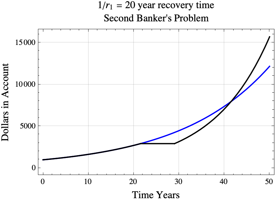
If you do purchase the interest rate hike at the optimal time, how many years will you need to wait until the optimal strategy surpasses the never buy strategy. The recovery time for the second banker’s problem is almost, but not quite the same as the first banker’s problem. For the second banker’s problem,
$$
t_{\mathrm{surpass}} = t_{buy} + 1/r_1.
$$
For the example,
$$
t_{\mathrm{surpass}} \approx 21.5228+ \frac{1}{0.05} = 41.5228.
$$

SecRecover

The black line shows the results of buying the interest rate increase at the optimal time. The blue line shows what happens if you never buy the interest rate hike and just continue to get 5% interest.
If you buy the interest rate hike at the optimal time, then you will maximize the account balance at all times $t>1/r_1$ years later. (Mathematically, for every $t> t_{\mathrm{buy}} + 1/r_1$, the strategy of purchasing the interest rate upgrade at time $t_{\mathrm{buy}}$ results in an account balance at time $t$ that exceeds the account balance at time $t$ using any other strategy.)
Erik Brynojolfsson, director of the MIT Center for Digital Business, gave a great TED talk on the recent changes in world-wide productivity, computers, machine learning and the “great stagnation“.  There has been a stagnation in GDP per capita for the last 5 years in the United States, Europe, and Japan.  However, growth has continued unabated in India, China, and Brazil.  Economist Tyler Cowen is not particularly optimistic about the current economic situation which he describes in his book “The Great Stagnation: How America Ate All The Low-Hanging Fruit of Modern History, Got Sick, and Will (Eventually) Get Better” ($4 Kindle edition). Erik disagrees with the idea that the economy, technology, and science are stagnant.  Instead, we are being confused by what he calls the “great decoupling” of productivity growth and employment/median income.  He believes that we are actually in the early phases of the “new machine age” which will create more wealth than the industrial revolution.  Here are some notes on his TED talk:

  • The introduction of electricity did not immediately lead to large productivity growth. At first, factory managers just replaced existing steam machines with electric machines. It took thirty years (one generation) before the factories were redesigned with electricity in mind and new work processes were created. Then productivity growth took off.
  • Big general purpose technologies like fire, agriculture, writing, metallurgy, printing press, steam engine, telecommunications & electricity, and now computers cause “cascades of complementary innovations”.
  • The GDP growth rate in America has been fairly steady at an average of 1.9% per year since 1800.
  • Erik graphically compares the 1960-2011 productivity growth caused partly by computers and the 1890-1940 productivity growth caused by electricity.  They appear quite similar.
  • Productivity has grown faster (2.4% per year) in the last decade than any other decade since 1970. The average productivity growth rate was about 2.3% during the second industrial revolution.
  • World GDP in the last decade has grown faster than any other decade in history.
  • New growth has been driven by thoughts and ideas more than physical products. This growth is hard to measure. The massive utility of free products like Google Search or the Wikipedia is not included in GDP.
  • The “new machine age” is “digital, exponential, and combinatorial”.
  • Digital goods are perfectly, freely replicable and they have near zero transportation cost (often moving at great speed crossing the globe in a minute.)
  • Computer power has grown exponentially. In Erik’s words, “Computers get better faster than anything else ever.” (2013 playstation = 1996 supercomputer)
  • We are not designed by evolution to anticipate exponential trends. We expect linear trends.
  • We now have Big Data and Machine Learning which allow us to analyze everything more deeply.
  • He disagrees with the idea of “low hanging fruit” inventions (see e.g. Cowen’s book). He thinks that “each innovation produces building blocks for even more innovations”.
  • The digital, exponential, and combinatorial nature of the new machine age will lead to the greatest industrial revolution in history. (see e.g. cat transportation at 6:55 in the video).
  • Machine Learning may be the most important innovation of this revolution. (The Watson Jeopardy team improved faster than any human could by using machine learning.)  Watson’s technology is now being applied in the legal, banking, and medical fields.
  • “The great decoupling” is the decoupling of high productivity growth from employment and median income.
  • Jobs are being replaced by computers.
  • In 1997 Gary Kasparov was beaten by the super computer Deep Blue. Today a cell phone can beat a chess grandmaster.
  • In computer assisted chess play (Advanced Chess), sometimes the winners are neither computer experts nor grandmasters. Instead, they were the best at interacting with the computer—guiding its exploration of the possibilities. So, maybe we will not lose our jobs to computers, rather we will collaborate with computers to create wonderful things.