A huge numbers of videos from PyCon 2012 Us are available at pyvideo.org. Marcel Caraciolo at aimotion.blogspot.com posted links to 17 of them on his blog. I have been avoiding Python for machine learning, but maybe I’ve been wrong.
In “How to Use Expert Advice“, Cesa-Bianchi, Freund, Haussler, Helmbold, Sharpire, and Warmuth (1997) describe boosting type algorithms to combine classifiers. They prove a bound of
$$ \sqrt{n \log(M)}$$
on the total regret where $n$ is the number of data points and $M$ is the number of classifiers. They relate their bounds to the L1 distance between binary strings and apply their results to pattern recognition theory and PAC learning.
In “Greedy Function Approximation: A Gradient Boosting Machine” Freeman(1999) presents an algorithm for incrementally improving the approximation of a function
$$f(x) = \sum_{m=0}^M \beta_m h(x, a_m)$$
where the $\beta_m$ are real and $a_m$ are a vectors of trained parameters. At each iteration, gradient boost adds on a new function $h$ using steepest descent.
Carl and I have been discussing concepts related to sparsity in neural nets. One older idea similar to sparsity is negatively correlated or uncorrelated neural nets. To use this technique, you could train several neural nets on part or all of the data and then keep the neural networks that are less correlated. The idea used CELS algorithm is to add a correlation penalty term to the loss function of the neural net optimization process. In “Simultaneous Training of Negatively Correlated Neural Networks in an Ensemble” Liu and Yao (1999) say that
The idea behind CELS is to encourage different individual networks in an ensemble to learn different parts or aspects of a training data so that the ensemble can learn the whole training data better.
which seems similar to what happens in sparse neural networks.
My Friend Andrew wrote:
Initially, I thought it was dependent on your definition of “random rational number”, but then I saw your second example that removed duplicates (1/2, 2/4, etc..).
I tried a different method by sampling from a real distribution and then rationalizing it:
Mean@Mod[Denominator@Rationalize[#, 1*^-6] & /@ RandomReal[{0, 1}, 100000], 2]Then, I tried changing the distribution, and still get the same result:
Mean@Mod[Denominator@Rationalize[#, 1*^-6] & /@ RandomReal[NormalDistribution[0, 1], 100000], 2]— Andrew

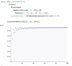
What percentage of “random fractions” have an even denominator? My friend Pig told me that the answer is around 1/3. (At least the answer is 1/3 for two somewhat natural definitions of the term “random fraction”.) Here is the experimental “proof” in Mathematica.
Mathematica input for test #1:
percentage[v_List, pred_] := N[ Length[Select[v, pred]] / Length[v] ]; percentage[ Table[ RandomInteger[{1, 1000}] / RandomInteger[{1, 1000}], {100000} ], EvenQ[Denominator[#]] ]
Output for test #1:
0.33343
Mathematica input for test #2:
percentage[ Table[i/j, {i, 1000}, {j, 1000}] // Flatten // Union, EvenQ[Denominator[#]] ]
Output for test #2 :
0.333443
Suppose some Intelligent Algorithm can learn to play tic-tac-toe. Tic-tac-toe is such a simple game that it can be exhaustively learned via memorization – but this is not what I mean here. I mean that the intelligent algorithm (IA) actually has the ability to generally learn, and that it has used this ability to learn tic-tac-toe. What would one like the IA to now know? Well, in addition to knowing the rules and optimal strategy of the game, the IA should also have figured out that tic-tac-toe is played on a planar grid, and that the winning positions correspond to horizontal, vertical, and diagonal lines on this grid.
Now after it has learned 3 x 3 tic-tac-toe, suppose that we want our IA to also learn to play 4 x 4 tic-tac-toe (perhaps this game should be called tic-toc-toe-tum). The IA should be able to use what it has learned in the 3 x 3 game to more easily learn the 4 x 4 game, and it should explicitly “understand” this relationship. Concretely, what does this mean?
I believe this is one of the couple fundamental open problems in machine learning.
I ran across an interesting paper yesterday “Logistic Regression, AdaBoost and Bregman Distances” (Collins, Schapire, Singer 2000). Adaboost is a great way to combine several weak predictors into a strong predictor (Freund 2012 is a great reference). The Bregman distance is a generalization of the Euclidean norm and KL-Divergence. Many well known algorithms that use the Euclidean norm still work when the Euclidian norm is replaced with a Bregman distance (e.g. Dykstra’s Algorithm see Censor Reich 2000). In the paper, the authors show that Adaboost solves a best approximation problem using the KL-distance and introduce many variants of Adaboost. Here are some quotes from the paper:
1) “We are now able to borrow methods from the maximum entropy literature for logistic regression and apply them to the exponential loss used by AdaBoost, especially convergence proof techniques.”
2) “Duffy and Helmbold (1999) gave conditions under which a loss function gives a boosting algorithm. They showed that minimizing logistic loss does lead to a boosting algorithm the PAC sense.”
3) “Our work builds heavily on that of Kivinen andWarmuth (1999) who, along with Lafferty, were the first to make a connection between AdaBoost and information geometry. They showed that the update used by AdaBoost is a form of “entropy projection.”” (bold face added.)
So, I am a bit disappointed that there do not seem to be any great methods for automated proving of theorems for games. The best seems to be “Automated Theorem Proving for General Game Playing” (Schiffel & Thielsche 2009) and “A Temporal Proof System for General Game Playing” (Thielscher & Voigt 2010). In the first paper, their program (which uses a sophisticated “answer set programming” theorem prover) proves theorems like ”
• proving that the argument of the control(P) feature is
unique in every state (provided the feature exists);
• proving that the contents of a board cell is unique (to which
end boards were identified manually);
• proving that the contents of a board cell is unique given
the information that the argument of control(P) is;
• proving that the game is zero-sum;
• systematic search for unique arguments as described at the
end of the preceding section.”
It is great that the authors combine automated theorem provers with game playing, but I am still somewhat disappointed because most people who play a game can easily read the rules and almost immediately answer questions about the game like “Is it zero-sum?” or “Do the squares only have one piece?”. I was hoping for deeper theorems. It is also disappointing that one of our best automated theorem proving algorithms cannot even prove these simple theorems for many games.
On the other hand, maybe we should only prove simple properties like this. When playing chess about the only theorems I ever apply are: 1) when in check, there are only three possible options – move the king, interpose a piece, or capture the attacking piece, and 2) if a piece is blocking an attack on its king, it cannot move (a pin). Really, I don’t think I use any theorems deeper than this while playing chess and those two theorems are not at all useful to a computer because the computer can easily list all the possible moves.
In other games, I guess I do use theorems like “if I lead the third highest card in bridge, a finesse will succeed if the player on my left has the second highest card and my partner has the highest card (assuming no trump)” or “if my team holds 11 of the hearts, then the other team’s hearts will split 1-1 52% of the time.”
If computers are going to reason about games, then we probably need fuzzy logic (as in this paper) and/or probability theory.