Games

You are currently browsing the archive for the Games category.

ROI in Games Part 2 – The Tank Game

February 26, 2023 in Games, Investing, Math by hundalhh | Permalink

Last month I wrote a post about the fact that you should not make an investment in a game that does not pay for itself. If an investment costs $I$ and gives you a return of $i$ per turn, then it will pay for itself in $I/i$ turns. The return on investment (ROI) is $$r= i/I.$$ In some games we have several choices about how to invest, and generally speaking it is best to choose the investments with the best ROI.

If you can invest on any turn, the ROI investment rule of thumb is,

“Don’t invest if there are less than $$I/i=1/r$$ turns in left in the game excluding the current turn.”

the tank game

The tank game is one of the simplest investment games. It illustrates a few common ideas in investment games:

Exponential Sharpening of the Axe
The optimal investment choice often depends only on the ROI for the turn and the number of turns left in the game.
Solving an investment game often involves finding the largest rectangle under the investment curve.
The investment-exploitation phase transition, dominating strategies, comparing two very similar strategies, null moves, and strategy swaps
Actually proving that a strategy is correct is a bit tricky.
Discrete vs. Continuous.

I will address some of these ideas in this post and the rest of the ideas in a follow up post.

Suppose that you start the game with an income of \$100 million per turn. Each turn you have the two choices:

(investment option) investing all your income into factories and increasing your income by 10%, or
(don’t invest option) building tanks that cost one million dollars each.

Assume that it is also possible to build half a tank, or any other fraction of a tank, so if you spend \$500,000 on tanks, you get 0.5 tanks. If you spend \$2,300,000 on tanks, then you get 2.3 tanks. The game lasts for 27 turns and the object of the game is to maximize the number of tanks created.

Intuitively, you want to build up your factories in the first part of the game (Invest/Growth phase), and then transition to making tanks in the later part of the game (Exploitation phase).

Suppose that you build factory equipment for the first 5 turns, and then spend 22 turns building tanks. After the first turn, you have \$110 million income (\$100 million original income plus \$10 million income due to the investment into factory equipment). After the second turn, your income would be \$121 million (\$110 million at the start of the turn plus \$11 million additional income due to investment). After the third turn you would have \$133,100,00 income, the fourth \$146,410,000 income, and finally, at the end of the 5th turn, your income would be \$161,051,000 per turn. If you then build tanks for 22 turns, then you would have $$22\cdot161.051 = 3543.122\ \ \mathrm{tanks}$$ at the end of the game.

The optimal strategy for the tank game using the rule of thumb

The easy way to find the optimal strategy is to apply the ROI investment rule of thumb. We should invest as long as there are more than $I/i=1/r$ turns in the game after the current turn. In the tank game, you increase your income by 10% if you invest, so $r=0.10$ and $$1/r=10\ \ \mathrm{turns.}$$ On turns 1 through 16 there are more than 10 turns left in the game, so you must invest on those turns. On turn 17, there are exactly 17 turns left in the game, so it does not matter whether or not you invest on that turn. On turns 18, 19, … 27, there are less than 10 turns left in the game, so on those turns, you need to build tanks.

If you do invest for 17 turns, then your income would be $$\mathrm{income} = (1.1)^{17}\cdot \ \$100,000,000= \$ 505,447,028.50$$ per turn. Then you could buy tanks for 10 turns giving you about 5054.47 tanks.

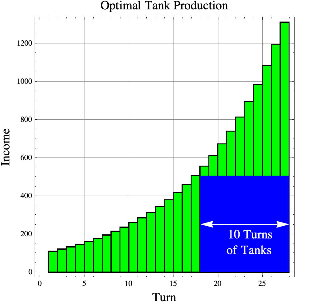
Notice that the amount of money spent on tanks is the same as the area of a rectangle with height equal to the income at the end of the investment phase (turn 17) times the number of turns used to buy tanks. Many investment problems are equivalent to finding the largest rectangle that “fits” under the income curve.

The investment-exploitation phase transition and dominating strategy swaps

If you actually want to prove that this is the optimal strategy, you should probably first prove that there is and investment phase followed by a building/exploitation phase.

We will prove that investment phase must come first by comparing two very similar strategies where we swap a Building action and an Investing action. Comparing two similar strategies and showing the one “dominates” the other is a common tactic for finding optimal strategies. In game theory, we say that one strategy dominates another if it is always better no matter what the opponent does. For the single player tank game, we will say that one strategy dominates another if it produces more tanks over the course of the game.

Option 1: Build-then-Invest. Suppose that on turn $i$ that you build tanks and on turn $i+1$ you invest in factories. Suppose that on turn $i$ that your income was $I$. Then you would build $$\mathrm{tanks} = \frac{I}{\$1,000,000}$$ tanks on turn $i$ and your income would increase to on turn $i+1$ to $$I_{\mathrm{new}}=1.1\ I.$$

Option 2: Invest-then-Build. On the other hand, if you swap the two strategies on turns $i$ and $i+1$, then on turn $i$ your income would again increase to $$I_{\mathrm{new}}=1.1\ I,$$ but when you build the tanks on turn $i+1$ you end up with $$\mathrm{tanks} = \frac{I_{\mathrm{new}}}{\$1,000,000}= \frac{1.1\ I}{\$1,000,000}.$$

For either option, you have the same income on turns $i+2, i+3, \ldots, 27$, but for Option 2 (Invest-then-build) you have 10% more tanks than option 1. We conclude that Option 2 “dominates” option 1, so for the optimal strategy, a tank building turn can never precede an investment turn. That fact implies that there is an investment phase lasting a few turns followed by an building phase where all you do is build tanks.

If we carefully apply the ideas in the ROI part 1 post, we can determine where the phase transition begins. Suppose that on turn $i$ we have income $I$ and we make our last investment to bring our income up to $1.1\ I$. The increase in income is $0.1\ I$ and that new income will buy $$\mathrm{tanks\ from\ new\ income} = \frac{0.1\ I (T-i)}{\$1,000,000}$$ new tanks where $T=27$ is the total number of turns in the game. If we build tanks instead of investing on turn $i$ then we would make $$\mathrm{potential\ tanks\ on\ turn\ }i = \frac{I}{\$1,000,000}$$ tanks. The difference is
$$\begin{aligned} \mathrm{gain\ by\ investing} &= \frac{0.1\ I (T-i)}{\$1,000,000}\; – \frac{I}{\$1,000,000}\\ &= \frac{0.1\ (T – i) \;- I}{\$1,000,000}.\end{aligned}$$

The gain is positive if and only if $$\begin{aligned} 0.1\ I (T-i) – I &> 0\\ 0.1\ I (T-i) &> I\\ 0.1\ (T-i) &> 1\\T-i &> 10\\T-10&> i.\end{aligned}$$

Remark: Reversing the inequalities proves that the gain is negative ( a loss) if and only if $T-10 < i$.

We conclude that no tanks can be built before turn $T-10=17$. On turn $i=17$, $$0.1\ I (T-i) -I = 0.1\ I (27-17) -I = 0,$$ so the gain by investing is zero. It does not matter whether the player builds tanks or invests on turn 17. After turn 17, the gain is negative by the Remark above, so you must build tanks after turn 17.

We have proven that the ROI investment rule of thumb works perfectly for the tank game.

ROI in Games – Part 1

January 14, 2023 in Games by hundalhh | Permalink

There are many games that have an investment phase followed by an exploitation phase including the card game Dominion, Terraforming Mars, Slay the Spire (during a combat), Saint Petersburg, Roll for the Galaxy, Master of Orion, Hansa Teutonica, Century Spice Road, Cash Flow and many more games.

One of the basic ideas is that you should not invest in something if there is not enough time for the investment to pay for itself.

A VERY SIMPLE HYPOTHETICAL GAME

Suppose that there are $T$ turns left in a game excluding the current turn, your current income level is I dollars per turn, and you have two choices:

(invest) Invest this turn to increase your income from $I$ dollars per turn to $I +i$ dollars per turn. You would then receive $I+i$ dollars per turn for the remaining $T$ turns for a total of $(I+i)\cdot T$ dollars.
(don’t invest) Receive $I$ dollars this turn and the remaining $T$ turns for a total of $(T+1)\cdot I$ dollars.

EXAMPLE

For example, assume that

it is currently turn 5,
at the start of turn 5 you have an income of $I$ = \$2 per turn,
the game ends on turn 9, and
you have the choice between two options:

Invest this turn to increase your income from \$2 per turn to \$3 dollars per turn. You would then receive \$3 dollars per turn for turns 6,7,8, and 9 for a total of \$3 * 4 = \$12 dollars.
Do not invest and you receive \$2 on this turn, turn 5, and the remaining turns 6,7,8, and 9, for a total of \$$2\cdot5$ = \$10 dollars.

For this example, $T=4$ because there are 4 remaining turns after the current turn. You have the option of increasing your income from \$2 to \$3, so the investment increases your income by $i$ = \$1 per turn.

The Correct Strategy

If you choose option 1, then your total earnings will be

invest_option_returns = $T\cdot (I+i)$ dollars.

If you choose option 2, then your total earnings will be

no_investment_option_returns = $(T+1)\cdot I$ dollars.

So, you should invest if

$$\begin{aligned}T\cdot (I+i) &> (T+1)\cdot I \\T\cdot I+T\cdot i &> T\cdot I + I \\T\cdot i &> I \\T&>\frac{I}{i}. \\\end{aligned}$$

So, according to the math above, you should not invest in something unless there are more than $$\frac{I}{i}= \frac1{r}$$ turns left in the game after the current turn where $$r=\frac{i}{I}$$ is sometimes called the return on investment (ROI).

When you invest $I$ dollars to get an increase of $i$ dollars per turn, it takes $I/i$ turns for the investment to “pay for itself”.

The Gain

If there are more than $\frac1{r}=\frac{I}{i}$ turns in the game, then you will gain

gain = invest_option_returns – no_investment_option_returns

$$\begin{aligned}&=T\cdot (I+i) – (T+1)\cdot I\\&=T I+T i – T i – I\\&= T i – I \\&= T r I – I \\&= (Tr -1) I \\&= I r \left(T -\frac1{r}\right) \end{aligned}$$

dollars by choosing to invest. The investment pays for itself after $1/r$ turns and every turn after that gives you $I r=i$ dollars.

APPLYING THE CORRECT STRATEGY TO THE EXAMPLE

For the example, $T=4, I=2,$ and $i=1$, so $r = i/I =0.5$. The correct strategy is to invest if

$$T > I/i,$$

but T=4 which is greater then I/i = 2, so the best option is the investment option.

I am hoping to write about applying this idea to several games over the next few weeks.

Optimal Putting in Disc Golf – Revised

April 23, 2022 in Games by hundalhh | Permalink

About a year ago, I posted a short article about optimal putting in disc golf. I gave an approximate rule of thumb to use at the end of the article, but it turns out that there is a better thumb rule, so I’m revising the post accordingly below.

I often have to make a decision when putting at the edge of the green during disc golf. Should I try to put the disc in the basket (choice 1) or should I just try to put the disc near the basket (choice 2)? If I try to put it in the basket and I miss, sometimes the disc will fly or roll so far way that I miss the next shot.

In order to answer this question, I created a simplified model. Assume:

If I do try to put it in the basket (choice 1), I will succeed with probability $p_1$.
If I do try to put it in the basket (choice 1), fail to get it in the basket, and then fail again on my second try, then I will always succeed on the third try.
If I don’t try to put the disc in the basket (choice 2), I will land near the basket and get it in the basket on the next throw.

Using these assumptions, I can compute the average number of throws for each choice.

For choice 2, I will always use two throws to get the disc in the basket.

For choice 1, there are three possible outcomes:

outcome 1.1: With probability $p_1$, I get it the basket on the first throw!
outcome 1.2: With probability $p_2$, I miss the basket, but get the disc in the basket on the second throw.
outcome 1.3: With probability $p_3$, I miss twice, and get it on the third throw.

I am assuming that if I miss twice, I will always get it on the third try, so

$$p_1 + p_2 + p_3=1.$$

Let $a$ be the average number of throws for choice 1. Then $$a = p_1\cdot 1 +p_2\cdot 2 +p_3\cdot 3.$$

I should choose choice 1 (go for it) if I average fewer throws than choice 2, i.e. if $a<2$. This occurs when

$$\begin{aligned}2 >& p_1\cdot 1 +p_2\cdot 2 +p_3\cdot 3 \\2 (p_1+p_2+p_3) >& p_1\cdot 1 +p_2\cdot 2 +p_3\cdot 3\\p_1\cdot 2+p_2\cdot 2+p_3\cdot 2 >& p_1\cdot 1 +p_2\cdot 2 +p_3\cdot 3\\ p_1 >& p_3.\end{aligned}$$

So, I should choose choice 1 if $p_1> p_3$. In words,

“Go for it if the probability of getting it on the first try is greater than the probability of missing twice”.

Optimal Putting in Disc Golf

May 20, 2021 in Games by hundalhh | Permalink

In order to answer this question, I created a simplified model. Assume:

If I don’t try to put the disc in the basket (choice 2), I will land near the basket and get it in the basket on the next throw.
If I do try to put it in the basket (choice 1), I will succeed with probability $p$, where $p$ depends only on distance to the basket.
If I do try to put it in the basket and fail to get it in the basket (choice 1), the probability that I will succeed on the second try is $q$ where $q$ is constant which does not depend on distance.
If I do try to put it in the basket (choice 1), fail to get it in the basket, and then fail again on my second try, then I will always succeed on the third try.

Using these assumptions, I can compute the average number of throws for each choice.

For choice 2, I will always use two throws to get the disc in the basket.

For choice 1, there are three possible outcomes:

outcome 1.1: I get it the basket on the first throw!
outcome 1.2: I miss the basket, but get the disc in the basket on the second throw.
outcome 1.3: I miss twice, and get it on the third throw.

The probabilities for each of those outcomes are: $p$, $(1-p) q$, and $(1-p)(1-q)$ respectively.

Let $a$ be the average number of throws for choice 1. Then $$\begin{aligned}a &= p\cdot 1 +(1-p)q\cdot 2 + (1-p)(1-q)\cdot 3 \\&= p + 2 q – 2 p q + 3 – 3 p – 3 q + 3 p q\\&=3 -2 p – q + p q.\end{aligned}$$

I should choose choice 1 if $ 2>a$. This occurs when

$$\begin{aligned} 2 &> 3 -2 p – q + p q\\-1 &> -2 p – q + p q \\-1 &> (q-2) p – q \\q -1 &> (q-2) p\\ \frac{q -1}{q-2} &< p \\\frac{1-q}{2-q} &< p. \\ \end{aligned}$$

Now you can plug in various values for $q$ to find the lowest value for $p$ needed to go for it.

Probability of Success          Required
 After Missing             Probability of Success
                             on the first try
     100%                           0%
      99%                           1%
      95%                           5%
      90%                           9%
      85%                          13%
      80%                          17%
      75%                          20%
      50%                          33%
      0%                           50%

So, if you are 100% certain that you will put it in the basket on the second try, then you should use choice 1 (going for it) if $p>0$ (i.e. always).

If you are 90% certain that you will put it in the basket on the second try, then you should use choice 1 (going for it) if $p>0.09=9\%$.

$$ $$

a rule of thumb

A nice approximate rule of thumb is to go for it if the sum of $p$ and $q$ is more than 100%.

When I am 6 yards from the basket, I will get it in about 75% of the time (p=0.75), and if I miss, I will usually get it in 90% of the time. The sum of 70% and 90% is 160%, so obviously, I should go for it.

When I am 9 yards from the basket, I will get it in about 20% of the time (p=0.20), and if I miss, I will usually get it in 85% of the time. The sum of 20% and 85% is 105%, so it seems like I should go for it.

If the basket is on a hill or if it is windy, then the disc will sometimes roll a fair distance if I miss. In that case, $q$ might be only 75%. The rule of thumb is that $p+q$ should be at least 100% to go for it, so according to the rule of thumb, I would need $p$ to be at least 25% to go for it. On a windy day, that’s like 6 yards for me.

A proof of Griffin’s Blackjack Theorem

April 17, 2021 in Games, Math by hundalhh | Permalink

Professor Peter Griffin discovered a nice theorem about the best way to count cards in Blackjack. (See the appendix in his book “Theory of Blackjack”). In this note, we review the theorem and reproduce his proof with more detail.

Suppose that you have a wagering game like blackjack which is played with a deck of cards. If you remove some cards from the deck, then the expected value of the game changes. Griffin found an easy formula for estimating the change in expectation caused by the removal of the cards. His formula depends on $E_j$ which is the change in expectation of the game when removing only the $j$th card from the deck.

Assume that the game never requires more than $k$ cards and the deck has $n$ cards in it. Obviously $n\geq k>0$. There are $m = {n \choose k}$ subsets of the deck $I_1, I_2, \ldots, I_m$ that contain $k$ cards each. Let $y_i$ be the expected value of the game played with the card subset $I_i$. We would like to estimate $y_i$ based on the cards in $I_i$.

We can create a linear estimate of $y_i$ by creating a vector $b=(b_1, b_2, \ldots, b_n)$ where $b_j$ is the “value” of the $j$th card. More specifically,
$$
y_i \approx \sum_{j\in I_i} b_j.
$$
Griffin found that the correct formula for $b_j$ is simply $$b_j = (\mu – (n-1) E_j)/k$$ where $\mu$ is the expected value of the game with a fresh deck. Using this value vector $b$ minimizes the squared error of the estimator. This formula is remarkable both for its simplicity and the fact that $k$ only plays a small roll in the calculation.

Griffin’s Theorem Let the error function $e:R^m \rightarrow R$ be defined as

$$
e(b) = \sum_{i=1}^m \left( y_i – \sum_{j\in I_i} b_j \right)^2 .
$$
Then $e(b^*) = \min_{b\in R^m} e(b)$ is the unique global minimum of $e$ where
$$
b^*_j = (\mu – (n-1) E_j)/k
$$
and $\mu$ is the expected value of the game with a fresh deck.

In the theorem above, $e$ is the sum of the squared errors in the linear estimate of the expected value of the game. In order to prove the theorem, we need two lemmas.

Lemma 1 If $\tilde{y}_j$ is the average expectation of the $k$ card subsets that do not contain card $j$, $\bar{y}_j$ is the average expectation of the $k$ card subsets that contain card $j$, and $\mu$ is the expectation of the game with a fresh deck, then
$$\mu = \frac{k}{n}\; \bar{y}_j + \left(1- \frac{k}{n}\right)\tilde{y}_j$$
and
$$\bar{y}_j = \frac{n \mu – (n-k) \tilde{y}_j}{k}.$$

The short proof of this lemma is left to the reader.

Lemma 2
Suppose for $j = 1,\ldots, n$,
$$(2.1)\quad b_j + \alpha \sum_{i=1}^n b_i = \gamma_j.$$ Then

$$ b_j = \gamma_j – \frac{\alpha\; n\; \bar\gamma}{1 + n \alpha}$$
where $\bar\gamma = \frac1n \sum_{j=1}^n \gamma_j$.

Proof: Sum both sides of equation (2.1) to get
$$
n \bar{b} + \alpha n^2 \bar{b} = n \bar{\gamma}
$$
where $\bar{b} = \frac1n \sum_{j=1}^n b_j$. Then,
$$
\begin{aligned}
\bar{b} + \alpha n \bar{b} &= \bar{\gamma} \\
\bar{b} &= \frac{\bar{\gamma}}{1+ n \alpha}.
\end{aligned}
$$
Applying that to equation (2.1) yields
$$
\begin{aligned}
b_j + \alpha \sum_{j=1}^n b_j &= \gamma_j \\
b_j + \alpha n \bar{b} &= \gamma_j\\
b_j + \alpha n \frac{\bar{\gamma}}{1+n \alpha} &= \gamma_j\\
b_j &= \gamma_j – \frac{\alpha\; n\; \bar{\gamma}}{1+n \alpha} \\
\end{aligned}
$$
which completes the proof of the Lemma.

Now we can prove Griffin’s Theorem.

Proof: Let the matrix $X$ be defined by $X_{ij} = 1$ if card $j$ is in set $I_i$ and $X_{ij}=0$ otherwise. We wish to minimize the sum of the squared errors. If we assume that the value of the $j$th card is $b_j$, then we can estimate the expectation of the game played using only card subset $I_i$ with
$$
\sum_{j\in I_i} b_j.
$$
The error of this estimate is $(y_i – \sum_{j\in I_i} b_j)$. The sum of the squared error is
$$
e(b) = \sum_{i=1}^m \left( y_i – \sum_{j\in I_i} b_j \right)^2.
$$
Noice that $\sum_{j\in I_i} b_j = x_i \cdot b$ where $x_i$ is the $ith$ row of $X$. So,
$$
e(b) = \sum_{i=1}^m \left( y_i – \sum_{j=1}^n X_{ij} b_j \right)^2 = \| X b – y \|^2.
$$
In other words $e(b)$ is the square of the distance between $y$ and $Xb$. The Gauss-Markov theorem provides a nice solution for the $b$ which minimizes this distance
$$
b^* = \left(X^T X\right)^{-1} X^T y
$$
where $X^T$ indicates the transpose of $X$. Hence,
$$
(1)\quad X^T X b^* = X^T y.
$$
Let $C=X^T X$. It turns out that $C$ has a very simple structure.

$C_{ij} = x_i^T x_j$ where $x_i$ and $x_j$ are the $i$th and $j$th columns of $X$, so
$$
(2) \quad C_{ii} = x_i^T x_i = { n-1 \choose k-1},
$$
and if $i \neq j$,
$$
(3)\quad C_{ij} = x_i^T x_j = { n-2 \choose k-2}.
$$

So, applying equations (2) and (3) to $i$th row of matrix equation (1) gives

$${n-1 \choose k-1} b_i^* + {n-2 \choose k-2} \sum_{j\neq i} b_j^* = {n-1 \choose k-1} {\bar{y}_i}$$
for $j=1, 2, \ldots n$ where $\bar{y}_j$ is the average expectation of the ${n-1\choose k-1}$ subsets with $k$ cards that contain card $j$.

Note that $$ {n-2 \choose k-2} / {n-1 \choose k-1} = \frac{k-1}{n-1} ,$$ so
$$
\begin{aligned}
b_i^* + \frac{k-1}{n-1} \sum_{j\neq i}^n b_j^* &= \bar{y}_i \\
b_i^* – \frac{k-1}{n-1} b_i^* + \frac{k-1}{n-1} \sum_{j=1}^n b_j^* &=\bar{y}_i \\
\frac{n-k}{n-1} b_i^* + \frac{k-1}{n-1} \sum_{j=1}^n b_j^* &= \bar{y}_i \\
(n-k) b_i^* + (k-1) \sum_{j=1}^n b_j^* &= (n-1) \bar{y}_i\\
b_i^* + \frac{k-1}{n-k} \sum_{j=1}^n b_j^* &= \frac{n-1}{n-k}\bar{y}_i.
\end{aligned}
$$
We apply Lemma 2 with $\alpha = \frac{k-1}{n-k}$ and $\gamma_j = \frac{n-1}{n-k} \bar{y}_j$ to get
$$
\begin{aligned}
b_j^* &= \gamma_j – \frac{\alpha\; n\; \bar\gamma}{1 + n \alpha} \\
&= \frac{n-1}{n-k} \bar{y}_j\; – \frac{\frac{k-1}{n-k}\; n\; \bar\gamma}{1 + n\; \frac{k-1}{n-k}} \\
&= \frac{n-1}{n-k} \bar{y}_j\; – \frac{(k-1) \; n\; \bar\gamma}{n-k + n(k-1)} \\
&= \frac{n-1}{n-k} \bar{y}_j\; – \frac{(k-1) \; n\; \bar\gamma}{n-k + n k-n} \\
&= \frac{n-1}{n-k} \bar{y}_j\; – \frac{(k-1) \; n\; \bar\gamma}{-k + n k} \\
&= \frac{n-1}{n-k} \bar{y}_j\; – \frac{(k-1) \; n\; \bar\gamma}{k (n-1)} \\
&= \frac{n-1}{n-k} \bar{y}_j\; – \frac{(k-1) \; n\; \frac{n-1}{n-k} \mu }{k (n-1)} \\
&= \frac{n-1}{n-k} \bar{y}_j\; – \frac{(k-1) \; n\; \mu }{(n-k)k}. \\
\end{aligned}
$$
By Lemma 1,
$$\bar{y}_j = \frac{n \mu – (n-k) \tilde{y}_j}{k},$$
so
$$
\begin{aligned}
b_j^*
&= \frac{n \mu – (n-k) \tilde{y}_j}{k} \frac{n-1}{n-k} – \frac{ n (k-1)\mu}{k (n-k)} \\
&= \frac{ n (n-1) \mu }{(n-k)k} – \frac{ (n-k) \tilde{y}_j (n-1)}{k(n-k)} – \frac{ n (k-1)\mu}{k (n-k)} \\
&= \frac{ n (n-1) \mu }{(n-k)k} – \frac{ n (k-1)\mu}{k (n-k)} – \frac{ (n-k) \tilde{y}_j (n-1)}{k(n-k)} \\
&= \frac{n \mu}{k} \left[ \frac{n-1}{n-k} - \frac{k-1}{n-k} \right] – \frac{ \tilde{y}_j (n-1)}{k} \\
&= \frac{n \mu}{k} – \frac{ \tilde{y}_j (n-1)}{k} \\
&= \frac{n \mu – (n-1) \tilde{y}_j}{k} \\
&= \frac{\mu – (n-1) (\tilde{y}_j- \mu)}{k} \\
&= \frac{\mu – (n-1) E_j}{ k }
\end{aligned}
$$
which completes the proof.

In the future, I hope to write some articles about how Griffin’s Theorem can be applied to other games.

I should mention that it is not too hard to extend Griffin’s Theorem to get more accurate quadratic approximation of the expectation of the game with card removal (or higher degree polynomial approximations).

A Simple Minesweeper Puzzle

February 8, 2021 in Games, Logic, Statistics by hundalhh | Permalink

Suppose that you are playing the game Minesweeper. On your first move, you click on the lower left corner square and reveal a 1. Then you click on the square above the corner and reveal a 2. Then you click on the square above that and reveal a 3. What is the “safest” next move?

In order to talk about the contents of the blue squares, we will label them A,B,C,D, and E.

There are only three possible scenarios:

a) A, B, C, and E have mines,

b) A, C, and D have mines, or

c) B, C, and D have mines.

But, not all of these scenarios are equally likely. Suppose there are a total of $m$ mines on the board and $s$ squares left excluding the eight that we are looking at. Then the total number of possible distributions of the mines for scenarios a, b, and c are:

$n_a = {s\choose m-4},$
$n_b= {s\choose m-3},$ and
$n_c ={s\choose m-3}.$

These scenarios are not equally likely. (Above we used choose notation. ${n\choose m}= \frac{n!}{m! (n-m)!}$ where $n!=1\cdot2\cdot3\cdot\cdots\cdot n$. For example 4!=24 and ${5\choose 2}=\frac{5!}{2!\ \cdot\ 3!} = \frac{120}{2 \cdot 6}= 10$.) In fact,

$$\begin{aligned} r=\frac{n_b}{n_a}&=\frac{s\choose m-3}{s\choose m-4} \\&=\frac{\frac{s!}{(m-3)! (s-(m-3))!}}{\frac{s!}{(m-4)! (s-(m-4))!}}\\&=\frac{\frac{1}{(m-3)! (s-(m-3))!}}{\frac{1}{(m-4)! (s-(m-4))!}}\\&= \frac{(m-4)! (s-(m-4))!}{(m-3)! (s-(m-3))!}\\&= \frac{ (s-m+4)!}{(m-3) (s-m+3))!}\\&= \frac{ s-m+4}{m-3 }.\end{aligned}$$

In the beginning of the game $r\approx s/m-1\approx 4$, so scenarios b and c are about four times as likely as scenario a. We can now estimate the probabilities of scenarios a, b, and c to be about

“probability of scenario a” = $p_a \approx 1/9,$
“probability of scenario b” = $p_b \approx 4/9, and$
“probability of scenario c” = $p_c \approx 4/9.$

We can now conclude that the probability that square A has a mine is 5/9, that square B has a mine is 5/9, that square C has a mine is 100%, that square D has a mine is 8/9, and that square E has a mine is 1/9, so square E is the “safest” move.

Generally speaking, scenarios with more mines are less likely if less than half of the unknown squares have mines.

Another interesting way to think about it is that the 3 and 2 squares pulled the mines toward them making square E less likely to contain a mine.

You can approximate the probability of each scenario by just assuming that the squares are independent random variables (a false, but almost true assumption) each of which has probability $m/s$ of containing a mine. Using that method gives the same results as the approximation above.

If you prefer an exact calculation, then use the formula

$$ r=\frac{ s-m+4}{m-3 }$$

to get the exact ratio of $\frac{p_b}{p_a} = \frac{p_c}{p_a}=r$.

(PS: Jennifer told me via email that you can play Minesweeper online at https://www.solitaireparadise.com/games_list/minesweeper.htm)

Analyzing Slay the Spire and Sharing the Analysis

October 11, 2020 in Games by hundalhh | Permalink

So, I have played about 300 hours of Slay the Spire since I got it on July 26. It’s a turn-based deck building game. Many of these deck building games have interesting mathematics, so I have been devoting a fair amount of time to analyzing the game and writing about the game.

The most interesting theorem about the game is

D = h (( d – c b + w)/a + b/alpha)

where D is the total damage that you take, h is the total amount of damage that you give to the enemy, d is the average attack per turn from the enemy, c is the average number of cards you play per turn, b is the average block per blocking card played, w is the average amount of waisted block per turn, and alpha is the average attack for the attack cards you played. (PDF slides here.)

The nice thing about the formula is that h, d, c, b, and alpha are often precisely known or easy to calculate. Also, a large portion of the reasonable strategies have w=0. If you know h,d,c,b, and w and they are constant, then the correct strategy is simple: if (d-c b + w) is positive, then don’t block. If it’s negative, then block a lot.

There are other analysis techniques that were mentioned in the Sept 27, 2020 reddit post “Simplified Spire Puzzles“. My favorite is looking at the ratio of damage received to damage given.

Also, I wrote a computer program that computes the best possible strategy for just about any Slay Spire combat situation. The drawback is that if you have over 20 cards and 10 different types of cards, the program needs about 10 terabytes of ram and 3 years of cpu time to computer the answer. It is much quicker if you have only 10 cards the are all strike or block cards in which case it takes less than one cpu second and only a few kilobytes of ram.

I have been wondering how to present this information to the world. Today, I showed the formula and my program to my friends Cat and Chuck who are both a) fans of Slay the Spire, and b) programmers. Additionally, I created about 10 power point slides and a 16 page document mostly describing simplified Slay the Spire problems and their solutions.

Additionally, I would like to document all the card combinations that result in either an infinite sequence of actions (resulting from hyperbolic growth) or another kind of growth. Growth in this game seems to be limited to quadratic (1 4 9 16 25…), cubic (1 8 27 64 125…), or exponential (1 2 4 8 16 32…). I have never seen any other kind of growth in any game except dominion which can have polynomial growth where the exponent is a fraction.

I don’t mind writing, but I do mind rewriting and combining my short essays into a larger, more useful work especially if no one is going to read it.

Cheers, Hein

AlphaGo is changing how the Game is Played

May 18, 2017 in Deep Belief Networks, Games, General ML, Neural Nets, Reinforcement Learning by hundalhh | Permalink

In March of 2016, the computer program AlphaGo defeated Lee Sedol, one of the top 10 Go players in the world, in a five game match. Never before had a Go computer program beaten a professional Go player on the full size board. In January of 2017, AlphaGo won 60 consecutive online Go games against many of the best Go players in the world using the online pseudonym Master. During these games, AlphaGo (Master) played many non-traditional moves—moves that most professional Go players would have considered bad before AlphaGo appeared. These moves are changing the Go community as professional Go players adopt them into their play.

Michael Redmond, one of the highest ranked Go players in the world outside of Asia, reviews most of these games on You Tube. I have played Go maybe 10 times in my life, but for some reason, I enjoy watching these videos and seeing how AlphGo is changing the way Go is played. Here are some links to the videos by Redmond.

Two Randomly Selected Games from the series of 60 AlphaGo games played in January 2017

https://www.youtube.com/watch?v=gWabLAkvpIQ

https://www.youtube.com/watch?v=G5OKn2lWICk

Match 1 – Google DeepMind Challenge Match: Lee Sedol vs AlphaGo
https://www.youtube.com/watch?v=vFr3K2DORc8

The algorithms used by AlphaGo (Deep Learning, Monte Carlo Tree Search, and convolutional neural nets) are similar to the algorithms that I used at Penn State for autonomous vehicle path planning in a dynamic environment. These algorithms are not specific to Go. Deep Learning and Monte Carlo Tree Search can be used in any game. Google Deep Mind has had a lot of success applying these algorithms to Atari video games where the computer learns strategy through self play. Very similar algorithms created AlphaGo from self play and analysis of professional and amateur Go games.

I often wonder what we can learn about other board games from computers. We will learn more about Go from AlphaGo in two weeks. From May 23rd to 27th, AlphaGo will play against several top Go professionals at the “Future of Go Summit” conference.

Cheers,
Hein

Counterfactual Regret Minimization

April 11, 2017 in Games, General ML, Reinforcement Learning by hundalhh | Permalink

Gettysburg University has a nice webpage on Counterfactual Regret. Counterfactual Regret was used by the University of Alberta to solve the heads up limit Holdem poker game. (See e.g. the pokernews.com article).

Newly Published “Deep Learning” Book by Ian Goodfellow, Yoshua Bengio, and Aaron Courville

April 7, 2016 in Deep Belief Networks, Games, Neural Nets by hundalhh | Permalink

The book “Deep Learning” by Ian Goodfellow, Yoshua Bengio, and Aaron Courville (associated with the Google Deep Mind Team) is available in HTML format.

http://www.deeplearningbook.org/

« Older entries § Newer entries »

Artificial Intelligence Blog