The book “Deep Learning” by Ian Goodfellow, Yoshua Bengio, and Aaron Courville (associated with the Google Deep Mind Team) is available in HTML format.
You are currently browsing the archive for the Games category.
Wired has a nice article about the two most brilliant moves in the historic match between AlphaGo and Lee Sedol.
http://www.wired.com/2016/03/two-moves-alphago-lee-sedol-redefined-future/
In case you had not gotten the news yet, the Go playing program AlphaGo (developed by the Deep Mind division of Google) has beaten Lee Se-dol who is among the top two or three Go players in the world. Follow the link below for an informative informal video describing AlphaGo and the victory.
http://www.theverge.com/2016/3/9/11184362/google-alphago-go-deepmind-result
Science magazine has a nice pregame report.
Hey, I just enrolled in Stanford’s General Game Playing Course. General game playing programs are programs that try to play almost any game after being given the rules. There is a yearly competition of general game playing programs at the AAAI conference. If you join the course, send me an email so that we can exchange ideas or notes. (my email address is hundal followed by “hh” at yahoo.com)
Cheers, Hein
The Daily Mail reports that the Computer Poker Research Group at the University of Alberta seems to have solved heads-up limit hold’em poker.
You can play against their AI online.
(My thanks to Glen for emailing me the story!)
Christopher Clark and Amos Storkey wrote an interesting nine page article titled “Teaching Deep Convolutional Neural Networks to Play Go”. Their deep neural network correctly predicted the moves of experts on a 19×19 Go about 44% of the time. The previous record was 41% by Wistuba and Schmidt-Thieme in 2012. Furthermore, the Clark Storkey network was able to “consistently defeat the well-known Go program GNU Go.” This is the first time that a neural network was able to perform nearly as well as one of the better hand coded programs. It is still not as good at the better UCT programs, but it moves much more quickly than the UCT programs. I imagine that if there were a blitz version of computer Go, the Clark Storkey AI might win a computer competition.
The article reviews other recent attempts to train a neural network to play Go. The Clark Storkey network resembled the Wistuba Schmidt-Thieme network, but it had more 19×19 convolutional layers and the authors added one fully connected layer at the top before the final move decision. Also, known symmetries of the solution were hard-coded. Interestingly, they found that convolution seemed to be required.
“We briefly experimented with non-convolutional networks but found them to be much harder to train, often requiring more epochs of training and the use of approximate second order gradient descent methods, while getting worse results.”
Later they describe their training methods and network architecture as follows
“Networks were trained with mini-batch gradient descent with a batch size of 128, using a learning rate of 0.01 for 7 epochs, and 0.05 for 2 epochs which took about a day on a Nvidia GTX 780 GPU.”
“The best network had one convolutional layer with 64 7×7 filters, two convolutional layers with 64 5×5 filters, two layers with 48 5×5 filters, two layers with 32 5×5 filters, and one fully connected layer.”
They estimate that their AI would probably have a ranking near 4-5 kyu.
Mnih, Kavukcuoglu, Silver, Graves, Antonoglon, Wierstra, and Riedmiller authored the paper “Playing Atari with Deep Reinforcement Learning” which describes and an Atari game playing program created by the company Deep Mind (recently acquired by Google). The AI did not just learn how to pay one game. It learned to play seven Atari games without game specific direction from the programmers. (The same learning parameters, neural network topologies, and algorithms were used for every game).
The 2600 Atari gaming system was quite popular in the late 1970’s and the early 1980’s. The games ran with only four kilobytes of RAM and a 210 x 160 pixel display with 128 colors. Various machine learning techniques have been applied to the old Atari games using the Arcade Learning Environment which precisely reproduces the Atari 2600 gaming system. (See e.g. “An Object-Oriented Representation for Efficient Reinforcement Learning” by Diuk, Cohen, and Littman 2008, ”HyperNEAT-GGP:A HyperNEAT-based Atari General Game Player” by Hausknecht, Khandelwal, Miikkulainen, and Stone 2012, “Application of TEXPLORE on Atari Games “ by Shung Zhang , ”A Neuroevolution Approach to General Atari Game Playing” by Hausknect, Lehman,” Miikkulalianen, and Stone 2014, and “Replicating the Paper ‘Playing Atari with Deep Reinforcement Learning’ ” by Korjus, Kuzovkin, Tampuu, and Pungas 2014.)
Various papers have been written on how computers can learn to pay the Atari games, but most of them used the abstract representations of objects on the screen within the emulator. The Mnih et al AI learned to play the games using only the raw 210 x 160 video and the score. It seems to be the first successful attempt to learn arcade gaming from raw video.
To learn from raw video, they first converted the video to grayscale and then downsampled/cropped to 84 x 84 images. The last four frames were used to determine actions. The 28224 input pixels were run through two hidden convolution neural net layers and one fully connected (no convolution) 256 node hidden layer with a single output for each possible action. Training was done with stochastic gradient decent using random samples drawn from a historical database of previous games played by the AI to improve convergence (This technique known as “experience replay” is described in “Reinforcement learning for robots using neural nets” Long-Ji Lin 1993.)
The objective function for supervised learning is usually a loss function representing the difference between the predicted label and the actual label. For these games the correct action is unknown, so reinforcement learning is used instead of supervised learning. The authors used a variant of Q-learning to train the weights in their neural network. They describe their algorithm in detail and compare it to several historical reinforcement algorithms, so this section of the paper can be used as a brief introduction to reinforcement learning.
The AI was trained to play seven games: Beam Rider, Breakout, Enduro, Pong, Q*bert, Seaquest, and Space Invaders. In six of the seven games, this general game learning algorithm outperformed all previously known reinforcement learning algorithms tested on those games and “surpasses a human expert on three” of the seven games.
Even if you are not into chess, I think you will enjoy reading about Caruana’s amazing performance at Sinquefield.
(The cast comes off my hand today. I will be able to type with both hands soon!)

Monte Carlo Tree Search (survey) is working rather well for Go.
So far we have only considered blind strategies and a simple greedy strategy based on maximizing our score on every move. The results were interesting because the blind cyclic strategy left-down-right-down did surprisingly well and we saw that a biased random strategy which strongly favored two orthogonal moves like left and down with a small amount of one other move like right outperformed all of the other biased random strategies.
If we want to do better, we need something more sophisticated than a blind strategy or pure, short-term, score greed.
The first approach used by game AI programmers in the olden days was to simply program in the ideas that the programmer had about the game into the game AI. If the programmer liked to put an X in the middle of a tic-tac-toe board, then he hard-wired that rule into the computer code. That rule alone would not be enough to play tic-tac-toe, so the programmer would then just add more and more decision rules based on his own intuition until there were enough rules to make a decision in every game situation. For tic-tac-toe, the rules might have been
- If you can win on your next move, then do it.
- If your opponent has two in a row, then block his win.
- Take the center square if you can.
- Take a corner square if it is available.
- Try to get two squares in a single row or column which is free of your opponent’s marks.
- Move randomly if no other rule applies.
Though this approach can be rather successful, it tends to be hard to modify because it is brittle. It is brittle in two ways: a new rule can totally change the behavior of the entire system, and it is very hard to make a tiny change in the rules. These kind of rule based systems matured and incorporated reasoning in the nineties with the advent of “Expert Systems“.
Long before the nineties, the first game AI programmers came up with another idea that was much less brittle. If we could just give every position a numerical rating, preferably a real number rather than an integer, then we can make small changes by adding small numbers to the rating for any new minor feature that we identify.
In tic-tac-toe, our numerical rating system might be as simple as:
- Start with a rating of zero
- Add 100 to the rating if I have won,
- Subtract 100 if my opponent has won or will win on his next move,
- Add 5 if I own the central square,
- Add 2 points for each corner square that I own,
- Add 1 point for every row, column, or diagonal in which I have two squares and my opponent has no squares.
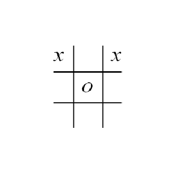
So, for example, the position below would be scored as
2 (for the upper left corner x) + 2 (for the other corner) + 1 (for the top row) = 5.
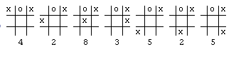
Now, in order to decide on a move, we could just look at every possible move, rate each of the resulting boards, and choose the board with the highest rating. If our tic-tac-toe position was the one below and we were the x player,

then we would have six possible moves. Each move could be rated using our board rating system, and the highest rated board with x in the center and a rating of 8 would be chosen.
$\ $
This approach was first applied to computer game AI by the famous theoretician Claude Shannon in the paper “Programming a Computer for Playing Chess” (1949), but the idea without the computers actually predates Shannon by hundreds of years. For instance, the chess theoretician Giambatista Lolli published “Osservazioni teorico-pratiche sopra il giuoco degli scacchi ossia il Giuoco degli Scacchi” in 1763. He was the first to publish the idea of counting pawns as 1, bishops as 3, knights as 3, rooks as 5, and queens as 9 thereby giving a rating to every board position in chess (well, at least a rating for the pieces). Shannon modified this rating by subtracting 0.5 for each “doubled” pawn, 0.5 for each “isolated” pawn, 0.5 for each “backward” pawn, and adding 0.1 for each possible move. Thus, if the pieces were the same for both players, no captures were possible, and if the pawns were distributed over the board in a normal fashion, Shannon’s chess AI would choose the move which created the most new moves for itself and removed the most moves from his opponent.
Shannon significantly improved on the idea of an evaluation function by looking more than one move ahead. In two players games, the main algorithm for looking a few moves ahead before applying the evaluation function is the alpha-beta search method which will be tested in a later post.
Let’s try to find and test a few evaluation functions for 2048.
Perhaps the simplest idea for evaluating a position is related to flying. According the great philosopher Douglas Adams,
“There is an art to flying, or rather a knack. Its knack lies in learning to throw yourself at the ground and miss. … Clearly, it is this second part, the missing, that presents the difficulties.” (HG2G).
Suffice it to say that in 2048, the longer you delay the end of the game (hitting the ground), the higher your score (the longer your flight). The game ends when all of the squares are filled with numbers, so if we just count every empty square as +1, then the board rating must be zero at the end of the game.
I ran 1000 simulated games with the Empty Tile evaluation function and got an average ending tile total of 390. The strategy ended the games with a maximum tile of 512 tile 25 times, a 256 tile 388 times, 128 491 times, 64 92 times, and 32 4 times.
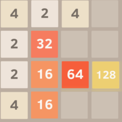
Well, that didn’t seem like anything spectacular. Let’s try to group like tiles—if there are two 128 tiles, let’s try to put them side-by-side. Of course, the idea of putting like tiles together is obvious. Slightly less obvious is the idea of trying to put nearly equal tiles together. Over at stackoverflow.com, the user ovolve, the author of the first 2048 AI, suggested the criteria of “smoothness” in his great post about how his AI worked. There are some interesting ways to measure smoothness with Fourier transforms, but just to keep things simple, let’s measure smoothness by totaling the differences between side-by-side tiles. For example, the smoothness of the board below would be
2+2+4 (first row) + 30+32 (second row) + 14+ 48 + 64 (third row) + 12 + 16 (fourth) + 2+0+2 (first col) + 30+16 + 0 (second) + 4 + 64 + 64 + 128 + 128
which sums to 662.
Once again I ran a 1000 games using smoothness as an evaluation function. The average ending tile total was 720, a new high. The strategy had a maximum ending tile total of 1024 3 times, 512 263 times, 256 642 times, 128 87 times, and 64 5 times. This looks very promising.
Let’s try ovolve’s last criteria — monotonicity. The idea of monotonicity is that we prefer that each row or column is sorted. On the board above, the top row
4 > 2 < 4 > 0 is not sorted. The second 2 < 32 > 0 = 0 and forth 4 < 16 > 0 = 0 rows are sorted only if the spaces are ignored. The third row 2 < 16 < 64 < 128 is fully sorted. Let’s measure the degree of monotonicity by counting how many times we switch from a less than sign to a greater than sign or vice-versa. For the first row we get 2 changes because the greater than sign 4 > 2 changed to a less than sign 2 < 4 and then changed again in 4 > 0. We also get two changes for 2 < 32 > 0, no sign changes in the third row (perfectly monotonic), and two changes in the last row.
I ran 100 games using the monotonicity evaluation function. The average ending tile total was 423. The maximum tile was 512 16 times, 256 325 times, 128 505 times, 64 143 times, and 32 11 times.
I have summarized the results of these three simple evaluation functions in the table below.
| Evaluation Func | AETT | Max Tile |
|---|---|---|
| Empty | 390 | 512 |
| Smoothness | 720 | 1024 |
| Monotonicity | 420 | 512 |
| Cyclic LDRD | 680 | 512 |
| Pure Random | 250 | 256 |
Well, clearly Smoothness was the best.
There are three great advantages to numerical evaluation functions over if-then based rules. One, you can easily combine completely different evaluation functions together using things like weighted averages. Two, you can plot the values of evaluation functions as the game proceeds, or even plot the probability of winning against one or two evaluation functions. Three, in 2048, there is the uncertainty where the next random tile will fall. With numerical evaluation functions, we can average together the values of all the possible boards resulting from the random tile to get the “expected value” (or average value) of the evaluation function after the random tile drop.
Well, that’s it for my introduction to evaluation functions. Next time we will focus on more sophisticated evaluation functions and the powerful tree search algorithms that look more than one move ahead.
Have a great day. – Hein