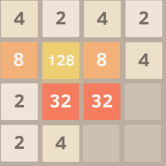
I will be continuing to post articles on AI for the game 2048.  The first two articles were:

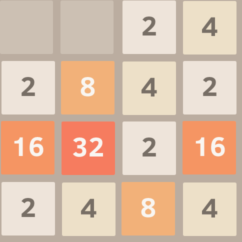
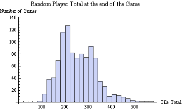
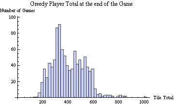
• An AI for 2048 — Part 1 – which described the game 2048 and reported the results of pure random play and a very simple greedy strategy that just tried to maximize it’s score on every move.
• An AI for 2048 — Part 2 Cyclic Blind Strategies – which reported on strategies that just cyclically repeated the same key stokes.

PROGRAMMING

In this article, I will make some comments on the cyclic blind strategies and report on random blind strategies.  The cyclic results can be generated from the Mathematica source code that I posted earlier.  The Biased Random results below can be obtained by just modifying the strategy function in the Mathematica source code.

CYCLIC BLIND

In the Cyclic Blind Article, we saw that left-down-right-down had the highest performance of any length 4 or less cyclic strategy with an average end tile total (AETT) of about 680.  The other cyclic strategies fell into the following seven groupings:

1. All four directions alternating vertical and horizontal (dlur, drul)  420 AETT.
2. All four directions without alternating vertical and horizontal (durl, dulr, dlru, …)  270 AETT.
3. Three directions with one direction repeated twice in a row where the directions that were not repeated were opposite (durr, dllu, dull, drru, …) 390 AETT
4. Three directions with one direction repeated twice in a row where the directions that were not repeated were perpendicular (drrl, duur, ddlu, …) 330 AETT
5. Three directions with one direction repeated, but not twice in a row, and the directions that were not repeated were perpendicular (dudr, duru, dldu …) 295 AETT
6. Three directions with no repetition (dlu, dur, …)  360 AETT
7. One Horizontal Direction + One vertical direction with or without repetition 60 AETT.

BLIND RANDOM BIASED STRATEGIES

The other blind strategy to consider is independent random biased selection of directions.  For example, someone might try rolling a six sided die and going left on 1, right on a 2 and down for rolls of 3, 4, 5, or 6.  I ran 1000 games each for every possible biased random strategy where the strategy was of the form

left with probability L/T, right with probability R/T,  up with probability U/T, down with probability D/T,

where T was the total of L, R, U, and D, and L, R, U and D between 0 and 4.

The results are tabulated below

AETT    MAX   
        TILE  L/T   R/T   U/T   D/T
11.138   16   1.    0.    0.    0.
55.416   128  0.57  0.    0.43  0.
56.33    128  0.67  0.    0.33  0.
57.17    64   0.5   0.    0.5   0.
57.732   128  0.6   0.    0.4   0.
70.93    16   0.6   0.4   0.    0.
71.246   32   0.57  0.43  0.    0.
71.294   32   0.5   0.5   0.    0.
71.752   32   0.67  0.33  0.    0.
234.42   256  0.4   0.4   0.1   0.1
238.182  256  0.38  0.38  0.12  0.12
241.686  256  0.44  0.33  0.11  0.11
245.49   256  0.44  0.44  0.11  0.
246.148  256  0.4   0.3   0.2   0.1
247.046  256  0.5   0.25  0.12  0.12
247.664  256  0.36  0.36  0.18  0.09
250.372  256  0.43  0.29  0.14  0.14
253.09   256  0.44  0.22  0.22  0.11
254.002  512  0.5   0.38  0.12  0.
255.178  256  0.33  0.33  0.22  0.11
255.242  256  0.33  0.33  0.17  0.17
255.752  256  0.33  0.33  0.25  0.08
257.468  512  0.43  0.43  0.14  0.
258.662  512  0.36  0.27  0.27  0.09
258.832  256  0.57  0.29  0.14  0.
258.9    256  0.36  0.27  0.18  0.18
260.052  256  0.3   0.3   0.2   0.2
261.676  256  0.38  0.25  0.25  0.12
261.902  256  0.31  0.31  0.23  0.15
262.414  256  0.27  0.27  0.27  0.18
263.702  256  0.27  0.27  0.27  0.2
264.034  256  0.31  0.23  0.23  0.23
264.17   512  0.57  0.14  0.14  0.14
264.2    256  0.29  0.29  0.29  0.14
264.226  256  0.31  0.23  0.31  0.15
264.232  256  0.29  0.29  0.21  0.21
264.33   256  0.5   0.17  0.17  0.17
265.328  256  0.33  0.22  0.22  0.22
265.512  256  0.4   0.2   0.3   0.1
265.724  256  0.4   0.2   0.2   0.2
265.918  512  0.33  0.25  0.25  0.17
265.986  256  0.3   0.3   0.3   0.1
266.61   256  0.25  0.25  0.25  0.25
266.796  256  0.29  0.21  0.29  0.21
266.812  256  0.31  0.31  0.31  0.08
267.096  256  0.33  0.17  0.33  0.17
267.5    512  0.33  0.25  0.33  0.08
267.804  256  0.36  0.18  0.27  0.18
267.99   256  0.3   0.2   0.3   0.2
268.414  512  0.43  0.14  0.29  0.14
268.634  256  0.44  0.11  0.33  0.11
271.202  256  0.38  0.12  0.38  0.12
271.646  256  0.33  0.22  0.33  0.11
271.676  512  0.5   0.33  0.17  0.
272.128  256  0.36  0.18  0.36  0.09
273.632  256  0.5   0.12  0.25  0.12
279.82   256  0.4   0.1   0.4   0.1
281.958  256  0.4   0.4   0.2   0.
291.702  512  0.44  0.33  0.22  0.
306.404  256  0.38  0.38  0.25  0.
306.508  512  0.5   0.25  0.25  0.
310.588  512  0.43  0.29  0.29  0.
310.596  512  0.36  0.36  0.27  0.
321.016  512  0.4   0.3   0.3   0.
333.788  512  0.33  0.33  0.33  0.
340.574  512  0.5   0.17  0.33  0.
341.238  512  0.57  0.14  0.29  0.
342.318  512  0.44  0.22  0.33  0.
347.778  512  0.36  0.27  0.36  0.
355.194  512  0.38  0.25  0.38  0.
366.72   512  0.5   0.12  0.38  0.
369.35   512  0.43  0.14  0.43  0.
371.63   512  0.4   0.2   0.4   0.
384.962  512  0.44  0.11  0.44  0.

There are a few things you might notice.

• The  best strategy was 44% Left, 11% Right, and 44% down with a AETT of 385 which was much better than pure random (25% in each direction), but not nearly as good as the cyclic strategy left-down-right-down (AETT 686).
• The AETT varies smoothly with small changes in the strategy.  This is not surprising.  You would think that 55% up, 45% down would have nearly the same result as 56% up and 44% down.  The Extreme value theorem then tells us that there must be a best possible random biased strategy.
• The top 17 strategies in the table prohibit one direction with AETTs of 280 to 385.
• If the strategy uses just two directions, then it does very poorly.

Well that’s it for blind strategies.  Over the next few posts, we will introduce evaluation functions, null moves, quiescent search, alpha-beta prunning, and expectimax search.

A guy named Phil asked me to post my code, so here it is.  It’s in Mathematica, so I imagine that most people will have trouble reading it.  I will probably rewrite the code in a more common, faster language later.

(* Mathematica code for simulating 2048
   - by Hein Hundal (Public Domain)

   Visit  http://gabrielecirulli.github.io/2048/

   for more detials.
*)

(* collapse[v] takes a list of values and returns a 
   collapsed list of values where two consecutive equal 
   values are summed into one value. *)

collapse[v_List] := PadRight[
   collapseAux[Cases[v, _Integer]]  , 4, "."];

collapseAux[{}] = {};
collapseAux[{x_}] = {x};
collapseAux[v_List] := If[ v[[1]] == v[[2]],
   Prepend[ collapseAux[Drop[v, 2]], v[[1]]*2],
   Prepend[ collapseAux[Drop[v, 1]], v[[1]]]];

vGlobalMoves = Characters["lrud"];
mGlobalEmptyBoard = Table[".", {4}, {4}];

move[mBoard_, sMove_String] := Switch[sMove,
   "l", collapse /@ mBoard,
   "r", Reverse /@ collapse /@ Reverse /@ mBoard,
   "u", Transpose[ collapse /@ Transpose[ mBoard ]],
   "d", Reverse[ Transpose[ 
        collapse /@ Transpose[ Reverse[ mBoard]]]],
   _, Throw[{"move::illeagal move", sMove}]];

(* game1Turn[ mStart_List, randFunc_, moveStrat_]
      Performs one turn of the game.
      - mStart is a 4 x4 game matrix where every elemet 
        is either a number 2, 4, 8, ... or the string ".".
      - randFunc is any function that take a positive 
        integer n as input and outputs a positive integer 
        between 1 and n.
      - moveStrat is any function that takes a game board as 
        an input and gives as an output one of the four 
        characters u, d, l, r.
      - The output of game1Turn is a new board state.  *)

game1Turn[ mStart_List, randFunc_, moveStrat_] :=
  Module[{sMove, mBoard, mEmpty, iSpot, iVal},
   sMove = moveStrat[mStart];
   mBoard = move[mStart, sMove];

   (* only add a new piece if the board changed *)
   If[ mBoard =!= mStart,
      mEmpty = Position[mBoard, "."];
      iSpot = randFunc[Length[mEmpty]];

      (* the new board tile will either be a 4 or a 2 *)
      iVal = If[ randFunc[10] == 1, 4, 2];
      mBoard = ReplacePart[mBoard, mEmpty[[iSpot]] -> iVal]
    ];
   mBoard];

(*  gameManyTurns  - executes iDo turns of the game  *)
gameManyTurns[mStart_List, randFunc_, moveStrat_, iDo_Integer] := 
   NestList[game1Turn[#, randFunc, moveStrat] &, mStart, iDo];

(******************* Display Results of Multiple Runs **********)

periodTo0[m_List]  :=  m /. "." -> 0;
maxTile[m_List]    := Max[Flatten[periodTo0[m]]]
totalTiles[m_List] := Total[Flatten[periodTo0[ m ]]];

rand1[i_Integer] := 1 + RandomInteger[i - 1];

(* rand2[m]   replaces a random entry on the board m with a 2 *)
rand2[m_List] := ReplacePart[ m, 
   (RandomInteger[3, {2}] + 1) -> 2];

runSeveralGames[ randFunc_, moveStrat_, iDo_Integer]  := 
   Module[{},
   Table[
    (* run a single game for 100 turns *)
    ten1 = gameManyTurns[rand2[mGlobalEmptyBoard], 
               randFunc, moveStrat, 100];

    (* keep going until there is not change for 50 moves *)
    While[ ten1[[-50]] =!= ten1[[-1]]  && Length[ten1] < 10000,
       ten1 =  Join[ten1, gameManyTurns[ten1[[-1]], 
                    randFunc, moveStrat, 100]]
    ];

    ten2 = TakeWhile[ ten1, # =!= ten1[[-1]] &];

    (* output a list {# turns of the game, tile Total,
    maximum tile} for each game *)
    {Length[ten2], totalTiles[Last[ten1]], maxTile[ten1[[-1]]]},
    {iDo}]];

stats[mRes_List] := Module[{mRN = N@mRes},
   {Mean[mRN], StandardDeviation[mRN], Max[mRes[[All, 3]]],
    Tally[mRes[[All, 3]]] // Sort}];

(******** Blind Cyclic Strategy ****************************)

(* createCyclicStrategy - creates a cyclic strategy function 
   from the string s.  If s = "uddl", then the strategy function 
   will repeat the sequence move up, move down, move down, and 
   move left indefinitely. *)

createCyclicStrategy[sMoves_String] := Module[
   {exHeld, iCount = 1},
   exHeld = Hold[
     Function[ m, chars[[ Mod[iCount++, iStringLength] + 1]]]];
   ReleaseHold[
    exHeld /. {chars -> Characters[sMoves] ,
      iStringLength -> StringLength[sMoves]}]];

testOneStrategy[] := Module[{},
   stratDRDL = createCyclicStrategy["drdl"];
   mRes = runSeveralGames[rand1, stratDRDL, 100];
   stats[mRes]];

In my last post, I described how to play 2048 and reported the results of some simple simulations.  Namely, I reported the results of two very simple strategies:

• Random play will achieve an average ending tile total (AETT) of 252 and usually the highest tile will be a 64 tile or a 128 tile (about an 85% chance of ending with one of those).
• A pure greedy strategy where the player just tries to make the largest new tile possible results in an average ending tile total (AETT) of 399 and usually the highest tile will be a 128 tile or a 256 tile (about an 87% chance of ending with one of those).

Blind Strategies

Perhaps surprisingly, there are “blind” strategies that will do even better than the pure greedy strategy.  Blind strategies are strategies that ignore the current state of the board.  I tried two types of simple blind strategies “biased random” and “repeating sequences”.  I will summaries the results of the biased random trials in my next post.

The simplest repeating strategy would be just hitting the same key every time—down, down, down, ….   Of course that does not do well.  Nor would down, up, down, up, ….  So the simplest repeating strategy worth trying would be down, right, down, right or some other combination of horizontal and vertical moves.  I ran 100 games for every possible repeated sequence of two to four moves and found that the best of these sequences was down, right, down, left  or a version of that sequence in disguise.  The results are captured in the table below.

Notice that restricting your moves to only two out of the four possibilities does poorly.  The Down, Left, Down, Left… strategy had an average tile total of only 44.38 at the end of the game and that strategy never created a tile above 64.

The best strategies were down-right-down-left or that same strategy in disguise (dlul, dldr, and drur are really the same strategy).  Notice that this strategy does better than pure greedy which had an AETT of 399.

What would you do with 2880 cores?

Vasik Rajlich, author of the legendary chess program Rybka,  used them to show that chess champion Bobby Fisher was right about the chess opening King’s Gambit (see “A bust for King’s Gambit“) .

King’s Gambit

Vasik proved that King’s Gambit is a loss for white unless white plays 3. Be2 after black takes the pawn.  (In that case, it’s a draw.)  For the details, click on the link below.

http://en.chessbase.com/post/rajlich-busting-the-king-s-gambit-this-time-for-sure

Is it possible to compare the skill of Bobby Fisher and Emanuel Lasker? Several years ago Jeff Sonas improved upon the Elo chess rating system and then created the wonderful chess statistical analysis website Chessmetrics, but the ratings of the great players were still based upon how they played against their contemporaries. Mr. Sonas and I briefly discussed over email that it might be better if we could rate their play using computer chess engines.   Back then, the computer chess programs were not quite as strong as the best humans, but it would have been interesting. Well time has past and now Houdini and Rybka are significantly stronger than the best human player, the young Norwegian Magnus Carlsen.  Other people had the same idea for comparing the best chess players of all time and it seems that José Capablanca was one of the best if not the best chess player of all time.  The best analyses of this type were done by Guid and Bratko in “Computer Analysis of World Chess Champions” (2006) and “Using Heuristic-Search Based Engines for Estimating Human Skill at Chess” (2011). They have written several easy-to-read popular articles for Chess Base including:

• “The quality of play at the Candidates” (April 2013)
• “A computer program to identify beauty in problems and studies” (2012)
• “Using chess engines to estimate human skill” (2011)
• “Computers choose: who was the strongest player?” (2006)
• “Computer analysis of world champions” (2006)

Here is how they describe their method of rating the players. 

• The analysis of each game starts at move 12.
• The chess engine evaluates the best moves (according to the computer) and the moves played by the player.
• All engine’s evaluations are obtained at the same depth of search.
• The score is then the average difference between evaluations of the best moves and the moves played.
• If the player’s mistake (as seen by the engine) at particular move is greater than 3.00, the score for this particular move becomes 300 “centipawns” (to avoid unreasonably high penalties for gross mistakes).
• Moves where both the move played and the move suggested by the computer had an evaluation outside the interval [-2.00, 2.00], are discarded. (In clearly won positions players are tempted to play a simple safe move instead of a stronger, but risky one. Such “inferior” moves are, from a practical viewpoint, perfectly justified. Similarly, in lost positions players sometimes deliberately play an objectively worse move.)
• All the scores are given in “centipawns”.