In part 1, we defined the term strictly concave and introduced the theorem that if $f$ is strictly concave and $f(x)=f(x+1)$, then the integer(s) that maximize $f$ are exactly the set $\{\mathrm{floor}(x+1), \mathrm{ceil}(x)\}$ which is usually a set containing only one number $\mathrm{round}(x+1/2)$.

Parabolas

The simplest concave functions are parabolas with the vertex at the top.  All parabolas can be described by three real numbers $a$, $b$, and $c$, and the formula $y=a x^2 + b x + c$.  For strictly concave parabolas $a<0$.  For example, if $a=-2$, $b=3$, and $c=5$, then the function $y= f(x) = -2x^2 + 3 x +5$ is the parabola shown below.

If the vertex (shown above in blue) is above the x-axis, then the x-coordiante of the vertex can be computed by finding the points where the concave parabola crosses the x-axis (shown above in orange).  In our case, the parabola $y=f(x)$ crosses the x-axis when $0=y=f(x)$, or when $$\begin{aligned}0&= -2x^2 + 3 x +5\\0&=-(2x^2-3×-5)\\0&=-(2×-5)(x+1).\end{aligned}.$$ If $0=\alpha\cdot \beta$, then either $\alpha=0$ or $\beta=0$.  So, the parabola crosses the x-axis when either $0=2×-5$ or $0=x+1$ which means that it crosses when $x=5/2$ or $x=-1$.  Parabolas are symmetric about the vertical line going through the vertex, so the x-coordinate of the vertex is half way between the x-coordinates of the crossing points (a.k.a the roots of $f(x)$).  $$\begin{aligned} x_\mathrm{vertex} &= \frac{x_\mathrm{crossing1} + x_\mathrm{crossing2}}2\\&= \frac{ -1 +5/2}2\\&=\frac{3/2}2\\&=3/4.\end{aligned}$$

So the x-coordinate of the vertex is $x=3/4$.  This is also the real number that maximizes $f(w)$ over all real numbers $w$.

In general, the x-coordinates of the crossing points can be found with the quadratic formula  $$x=\frac{-b\pm\sqrt{b^2-4ac}}{2 a}.$$ The  $\pm$ sign means that one crossing can be found by replacing $\pm$ with + and the other can be found by replacing the $\pm$ with -.  But, if you have one number that is $x_1=\alpha+\beta$ and another that is $x_2=\alpha-\beta$, then the average of the two numbers is just $\alpha$.  In other words if the two values of $x$ are $x=\alpha\pm\beta$, then the average value is just $\alpha$.  So, to computer the average x-coordinate of the crossing points, all we have to do is remove the $\pm$ sign and whatever it is applied to from the quadratic formula.  $$ x_\mathrm{vertex} = \frac{-b}{2 a}.$$

theorem #2

Informally, if $y=f(x)$ is a parabola, $f(x) = a x^2 + b x + c$, and $a<0$, then the integer(s) that maximize $f(x)$ are the set $\{\mathrm{floor}(x+1/2), \mathrm{ceil}(x-1/2)\}$ where $x=\frac{-b}{2 a}$.

If $x$ is an integer plus 1/2 (e.g. 2.5, 7.5, …), this set has two elements $x+1/2$ and $x-1/2$.  If $x$ is not an integer plus 1/2, the set has only one element $\mathrm{round}(x)$ and that is the integer that produces the highest possible value of $f(z)$ among all integers $z$.

examples

Example 1: If $f(x)= -2x^2 + 3 x +5$, then $a=-2$, $b=3$, and $c=5$.  The values of $x$ in the theorem is the same as the x-coordinate of the vertex $$x=\frac{-b}{2a} = \frac{-3}{2\cdot(-2)}= \frac{-3}{-4}=3/4.$$ The integer(s) that maximize $f(z)$ among all integers $z$ are the set  $$\begin{aligned}\{\mathrm{floor}(x+1/2), \mathrm{ceil}(x-1/2)\}&= \{\mathrm{floor}(3/4+1/2), \mathrm{ceil}(3/4-1/2)\}\\&= \{\mathrm{floor}(5/4), \mathrm{ceil}(1/4)\}\\&=\{1\}.\end{aligned}$$

Example 2: If we lower the parabola from example 1 by a little bit setting $f(x)= -2x^2 + 3 x +\sqrt{17}$, then $a=-2$, $b=3$, and $c=\sqrt{17}$.  The value of $x$ in the theorem is the same as the x-coordinate of the vertex $x=\frac{-b}{2a} =3/4.$  The result does not depend on $c$, so as in example 1, the integer that maximizes $f(z)$ among all integers $z$ is $z=\mathrm{round}(3/4)=1$.

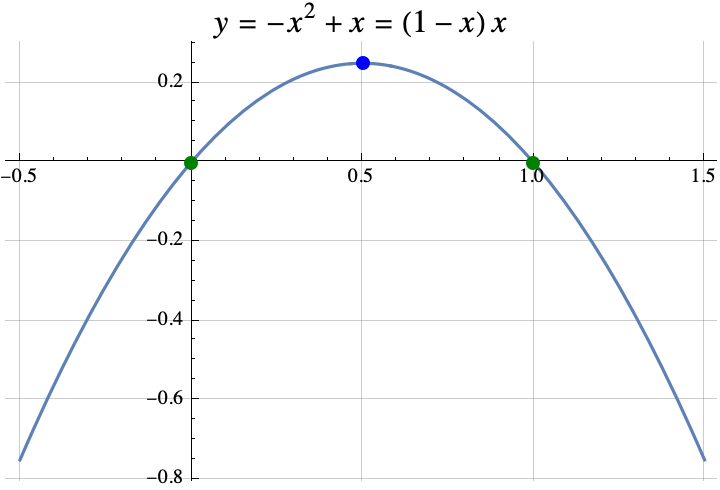
Example 3: $f(x)= -x^2+x = (1-x)x$, then $a=-1$, $b=1$, and $c=0$.  The value of $x$ in the theorem is the same as the x-coordinate of the vertex $$x=\frac{-b}{2a} =\frac{-1}{2\cdot (-1)}=1/2.$$ The integer(s) that maximize $f(z)$ among all integers $z$ are the set  $$\begin{aligned}\{\mathrm{floor}(x+1/2), \mathrm{ceil}(x-1/2)\}&= \{\mathrm{floor}(1/2+1/2), \mathrm{ceil}(1/2-1/2)\}\\&= \{\mathrm{floor}(1), \mathrm{ceil}(0)\}\\&=\{1,0\}.\end{aligned}$$ The integers that maximize $f(z)$ among all integers $z$ are 0 and 1.  If we look at the graph of $f(x)$ below, we can see that the graph crosses the x-axis at $x=0$ and $x=1$.  So, $f(0)=f(1)=0$.  All other integers inputs produce negative values.

the spirit of the proof

It turns out that Theorem 2 can be proven from theorem 1.  Recall that in Theorem 1, we wanted to find the value of $x$ where $f(x)=f(x+1)$.  If we found that value, then the integer(s) that maximize $f$ are exactly the set $\{\mathrm{floor}(x+1), \mathrm{ceil}(x)\}$.  In Theorem 2, $f(x) = a x^2 + b x + 1$.  So if $f(x)=f(x+1)$, then $$\begin{aligned}a x^2 + b x + c &= a (x+1)^2 + b (x+1) + c\\a x^2 + b x &= a (x+1)^2 + b (x+1)\\  a x^2 + b x &= a (x^2+2x+1)+ b x+b\\   a x^2  &= a x^2+2ax+a+ b \\    0  &= 2ax+a+ b \\ -a-b  &= 2ax \\ \frac{-a-b}{2a}  &= x\\ \frac{-b}{2a}-\frac12  &= x\\\end{aligned}.$$

Thus the integers that maximize $f(x)$ must be $$\begin{aligned} \{\mathrm{floor}(x+1), \mathrm{ceil}(x)\ \}&= \{\mathrm{floor}(\frac{-b}{2a}-\frac12+1), \mathrm{ceil}(\frac{-b}{2a}-\frac12)\} \\ &= \{\mathrm{floor}(\frac{-b}{2a}+\frac12), \mathrm{ceil}(\frac{-b}{2a}-\frac12)\}.\end{aligned}$$

Why DId I WANTED to know this

I was looking at several games where the optimal strategy depended on finding an integer $t$ that maximized $f(t)$.  In the game Slay the Spire, I wanted to maximize the amount of poison damage that I was going to do with the cards “Noxious Fumes” and “Catalyst”.  If I played the “Catalyst” on turn $t$ and the combat ended on turn $T$, then the poison damage done was $$\frac{(t+1)t}{2} -1 + (T-t)t$$ where  $ \frac{(t+1)t}{2}-1$ (note the triangle number) was the damage done by  “Noxious Fumes” and $ (T-t)t$ was the additional damage done by playing the Catalyst.  I wanted to maximize $f(t) = (T-t)t = -t^2 + T t$.

Using Theorem 2, $a=-1$, $b=T$, and $c=0$.  The Theorem says that the maximum damage occurs when you play the “Catalyst” on round $t$ where $t$ is contained in the set $\{\mathrm{floor}(x+1/2), \mathrm{ceil}(x-1/2)\}$ with $x=\frac{-b}{2 a}$.  So $x=\frac{-T}{2\cdot(-1)}=T/2$.  The best time to play the Catalyst was around half way through the combat. The catalyst should be played on round $T/2$ if $T$ is even.  If $T$ is odd, then the best round to play the “Catalyst” was for $t$ in the set $$\{\mathrm{floor}(T/2+1/2), \mathrm{ceil}(T/2-1/2)\}= \{\frac{T+1}{2}, \frac{T-1}{2} \}.$$

summary

So the first two theorems formalized two rules of thumb:

1. If you can find an $x$ where $f(x)=f(x+1)$, then the optimal integer(s) is $z=\mathrm{round}(x+1/2)$ with a special round that provides two answers if $x$ is an integer, and
2. If $f(x)=a x^2 + b x + c$ (a parabola), then the optimal integer(s) is $z=\mathrm{round}(x)$ where $x=\frac{-b}{2 a}$ which is the $x$ that maximizes $f(w)$ over all real numbers $w$ (i.e. the x-coordinate of the vertex).

If you want to see a more formal mathematical writeup, click here.

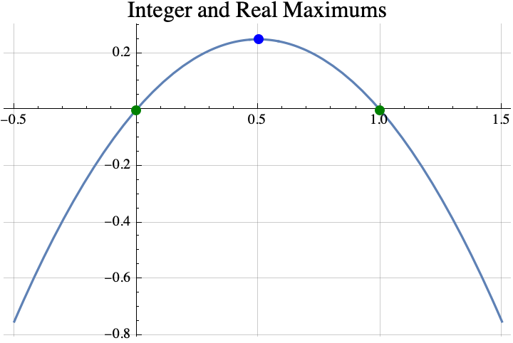
I proved a few simple but interesting theorems about integers that maximize a function $f$ when $f$ is a strictly concave function that maps real numbers to real numbers.  For example, the real number that maximizes $f(x)=x(1-x)$ is $x=1/2$, but among all the integers, the maximum possible value of the function is 0. And that maximum is achieved twice with integers 0 and 1, $f(0)=0=f(1)$.

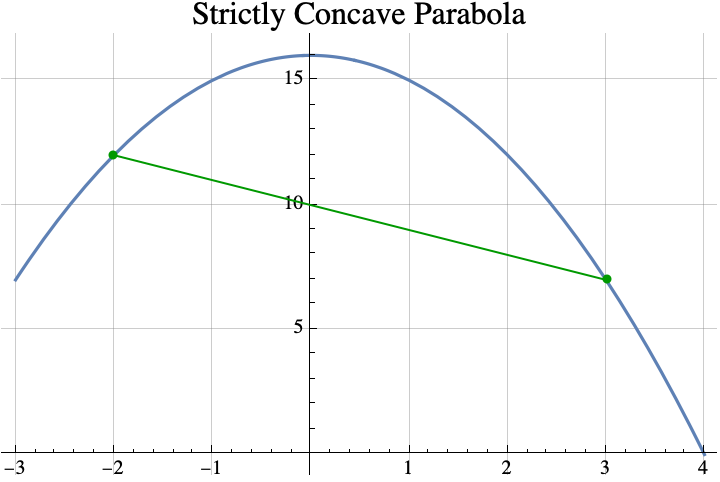
A function is strictly concave if you can pick any two points on its graph, draw a line between them, and the curve $y=f(x)$ between the two points lies entirely above the line between the two points.

Theorem #1

Informally stated, the first theorem is that if you can find a real number $x$ such that $f(x)=f(x+1)$, then the integer(s) that maximize the concave function $f$ are the set $\{\mathrm{floor}(x+1), \mathrm{ceil}(x)\}$ where “floor” just means round down and “ceil” means round up.  That set usually contains only one element which is $\mathrm{round}(x+1/2)$, but if $x$ is an integer, then it will contain two consecutive integers $x$ and $x+1$.

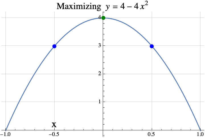
For example, if $f(x) = 4-4x^2$, then the value of $x$ that satisfies $f(x)=f(x+1)$ is $x=-1/2$ because $f(-1/2)=3=f(1/2)$.  So the theorem says that any integer that maximizes $f$ must be in the set  $$\begin{aligned}\{\mathrm{floor}(x+1), \mathrm{ceil}(x)\} &= \{\mathrm{floor}(-1/2+1), \mathrm{ceil}(-1/2)\}\\&= \{\mathrm{floor}(1/2), \mathrm{ceil}(-1/2)\} \\&= \{0\}.\end{aligned}$$ The integer that does the best is 0 which is also the real number that maximizes $f$.

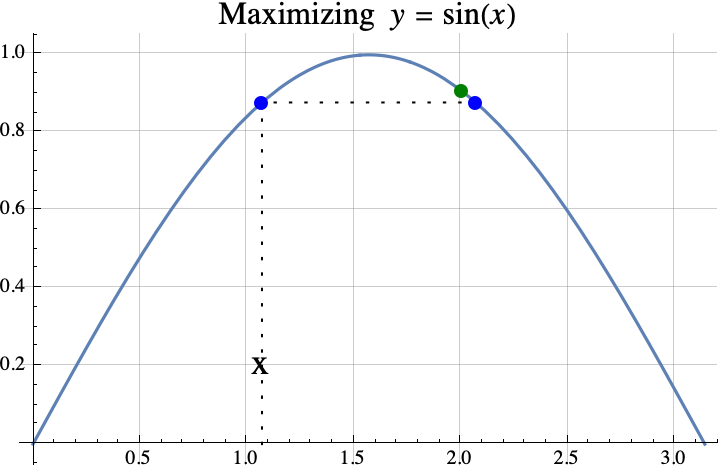
Here is another example.  If $f(x) = \sin(x)$, then the value of $x$ that satisfies $f(x)=f(x+1)$ is $x=1.0708$ because $f(1.0708)=0.877583=f(2.0708)$.  So the theorem says that any integer that maximizes $f$ must be in the set  $$\begin{aligned}\{\mathrm{floor}(x+1), \mathrm{ceil}(x)\} &= \{\mathrm{floor}(1.0708+1), \mathrm{ceil}(1.0708)\}\\&= \{\mathrm{floor}(2.0708), \mathrm{ceil}(1.0708)\} \\&= \{2\}.\end{aligned}.$$  The integer that does the best is 2.

So, that was the first theorem.  In part 2, we state a second theorem about finding the integer which maximizes a quadratic with some examples and one application the game “Slay the Spire”.

If you want to see a more formal mathematical writeup, click here.