Articles by hundalhh

Mathematician and Father. Into games, astronomy, psychology and philosophy.

Maximizing a function over integers (Part 2)

December 26, 2020 in Math, Optimization by hundalhh | Permalink

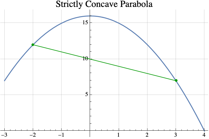
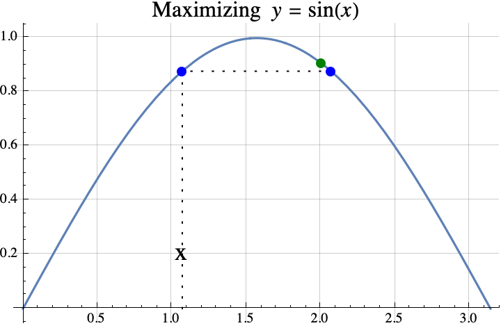
In part 1, we defined the term strictly concave and introduced the theorem that if $f$ is strictly concave and $f(x)=f(x+1)$, then the integer(s) that maximize $f$ are exactly the set $\{\mathrm{floor}(x+1), \mathrm{ceil}(x)\}$ which is usually a set containing only one number $\mathrm{round}(x+1/2)$.

Parabolas

The simplest concave functions are parabolas with the vertex at the top. All parabolas can be described by three real numbers $a$, $b$, and $c$, and the formula $y=a x^2 + b x + c$. For strictly concave parabolas $a<0$. For example, if $a=-2$, $b=3$, and $c=5$, then the function $y= f(x) = -2x^2 + 3 x +5$ is the parabola shown below.

If the vertex (shown above in blue) is above the x-axis, then the x-coordiante of the vertex can be computed by finding the points where the concave parabola crosses the x-axis (shown above in orange). In our case, the parabola $y=f(x)$ crosses the x-axis when $0=y=f(x)$, or when $$\begin{aligned}0&= -2x^2 + 3 x +5\\0&=-(2x^2-3×-5)\\0&=-(2×-5)(x+1).\end{aligned}.$$ If $0=\alpha\cdot \beta$, then either $\alpha=0$ or $\beta=0$. So, the parabola crosses the x-axis when either $0=2×-5$ or $0=x+1$ which means that it crosses when $x=5/2$ or $x=-1$. Parabolas are symmetric about the vertical line going through the vertex, so the x-coordinate of the vertex is half way between the x-coordinates of the crossing points (a.k.a the roots of $f(x)$). $$\begin{aligned} x_\mathrm{vertex} &= \frac{x_\mathrm{crossing1} + x_\mathrm{crossing2}}2\\&= \frac{ -1 +5/2}2\\&=\frac{3/2}2\\&=3/4.\end{aligned}$$

So the x-coordinate of the vertex is $x=3/4$. This is also the real number that maximizes $f(w)$ over all real numbers $w$.

In general, the x-coordinates of the crossing points can be found with the quadratic formula $$x=\frac{-b\pm\sqrt{b^2-4ac}}{2 a}.$$ The $\pm$ sign means that one crossing can be found by replacing $\pm$ with + and the other can be found by replacing the $\pm$ with -. But, if you have one number that is $x_1=\alpha+\beta$ and another that is $x_2=\alpha-\beta$, then the average of the two numbers is just $\alpha$. In other words if the two values of $x$ are $x=\alpha\pm\beta$, then the average value is just $\alpha$. So, to computer the average x-coordinate of the crossing points, all we have to do is remove the $\pm$ sign and whatever it is applied to from the quadratic formula. $$ x_\mathrm{vertex} = \frac{-b}{2 a}.$$

theorem #2

Informally, if $y=f(x)$ is a parabola, $f(x) = a x^2 + b x + c$, and $a<0$, then the integer(s) that maximize $f(x)$ are the set $\{\mathrm{floor}(x+1/2), \mathrm{ceil}(x-1/2)\}$ where $x=\frac{-b}{2 a}$.

If $x$ is an integer plus 1/2 (e.g. 2.5, 7.5, …), this set has two elements $x+1/2$ and $x-1/2$. If $x$ is not an integer plus 1/2, the set has only one element $\mathrm{round}(x)$ and that is the integer that produces the highest possible value of $f(z)$ among all integers $z$.

examples

Example 1: If $f(x)= -2x^2 + 3 x +5$, then $a=-2$, $b=3$, and $c=5$. The values of $x$ in the theorem is the same as the x-coordinate of the vertex $$x=\frac{-b}{2a} = \frac{-3}{2\cdot(-2)}= \frac{-3}{-4}=3/4.$$ The integer(s) that maximize $f(z)$ among all integers $z$ are the set $$\begin{aligned}\{\mathrm{floor}(x+1/2), \mathrm{ceil}(x-1/2)\}&= \{\mathrm{floor}(3/4+1/2), \mathrm{ceil}(3/4-1/2)\}\\&= \{\mathrm{floor}(5/4), \mathrm{ceil}(1/4)\}\\&=\{1\}.\end{aligned}$$

Example 2: If we lower the parabola from example 1 by a little bit setting $f(x)= -2x^2 + 3 x +\sqrt{17}$, then $a=-2$, $b=3$, and $c=\sqrt{17}$. The value of $x$ in the theorem is the same as the x-coordinate of the vertex $x=\frac{-b}{2a} =3/4.$ The result does not depend on $c$, so as in example 1, the integer that maximizes $f(z)$ among all integers $z$ is $z=\mathrm{round}(3/4)=1$.

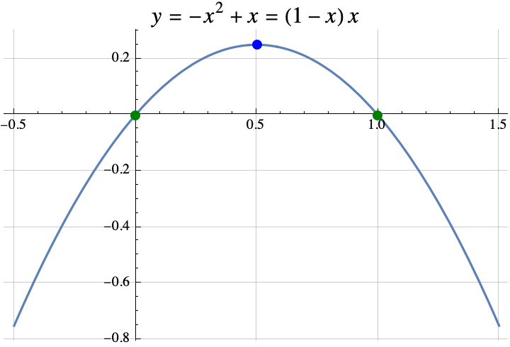
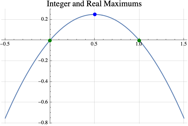
Example 3: $f(x)= -x^2+x = (1-x)x$, then $a=-1$, $b=1$, and $c=0$. The value of $x$ in the theorem is the same as the x-coordinate of the vertex $$x=\frac{-b}{2a} =\frac{-1}{2\cdot (-1)}=1/2.$$ The integer(s) that maximize $f(z)$ among all integers $z$ are the set $$\begin{aligned}\{\mathrm{floor}(x+1/2), \mathrm{ceil}(x-1/2)\}&= \{\mathrm{floor}(1/2+1/2), \mathrm{ceil}(1/2-1/2)\}\\&= \{\mathrm{floor}(1), \mathrm{ceil}(0)\}\\&=\{1,0\}.\end{aligned}$$ The integers that maximize $f(z)$ among all integers $z$ are 0 and 1. If we look at the graph of $f(x)$ below, we can see that the graph crosses the x-axis at $x=0$ and $x=1$. So, $f(0)=f(1)=0$. All other integers inputs produce negative values.

the spirit of the proof

It turns out that Theorem 2 can be proven from theorem 1. Recall that in Theorem 1, we wanted to find the value of $x$ where $f(x)=f(x+1)$. If we found that value, then the integer(s) that maximize $f$ are exactly the set $\{\mathrm{floor}(x+1), \mathrm{ceil}(x)\}$. In Theorem 2, $f(x) = a x^2 + b x + 1$. So if $f(x)=f(x+1)$, then $$\begin{aligned}a x^2 + b x + c &= a (x+1)^2 + b (x+1) + c\\a x^2 + b x &= a (x+1)^2 + b (x+1)\\ a x^2 + b x &= a (x^2+2x+1)+ b x+b\\ a x^2 &= a x^2+2ax+a+ b \\ 0 &= 2ax+a+ b \\ -a-b &= 2ax \\ \frac{-a-b}{2a} &= x\\ \frac{-b}{2a}-\frac12 &= x\\\end{aligned}.$$

Thus the integers that maximize $f(x)$ must be $$\begin{aligned} \{\mathrm{floor}(x+1), \mathrm{ceil}(x)\ \}&= \{\mathrm{floor}(\frac{-b}{2a}-\frac12+1), \mathrm{ceil}(\frac{-b}{2a}-\frac12)\} \\ &= \{\mathrm{floor}(\frac{-b}{2a}+\frac12), \mathrm{ceil}(\frac{-b}{2a}-\frac12)\}.\end{aligned}$$

Why DId I WANTED to know this

I was looking at several games where the optimal strategy depended on finding an integer $t$ that maximized $f(t)$. In the game Slay the Spire, I wanted to maximize the amount of poison damage that I was going to do with the cards “Noxious Fumes” and “Catalyst”. If I played the “Catalyst” on turn $t$ and the combat ended on turn $T$, then the poison damage done was $$\frac{(t+1)t}{2} -1 + (T-t)t$$ where $ \frac{(t+1)t}{2}-1$ (note the triangle number) was the damage done by “Noxious Fumes” and $ (T-t)t$ was the additional damage done by playing the Catalyst. I wanted to maximize $f(t) = (T-t)t = -t^2 + T t$.

Using Theorem 2, $a=-1$, $b=T$, and $c=0$. The Theorem says that the maximum damage occurs when you play the “Catalyst” on round $t$ where $t$ is contained in the set $\{\mathrm{floor}(x+1/2), \mathrm{ceil}(x-1/2)\}$ with $x=\frac{-b}{2 a}$. So $x=\frac{-T}{2\cdot(-1)}=T/2$. The best time to play the Catalyst was around half way through the combat. The catalyst should be played on round $T/2$ if $T$ is even. If $T$ is odd, then the best round to play the “Catalyst” was for $t$ in the set $$\{\mathrm{floor}(T/2+1/2), \mathrm{ceil}(T/2-1/2)\}= \{\frac{T+1}{2}, \frac{T-1}{2} \}.$$

summary

So the first two theorems formalized two rules of thumb:

If you can find an $x$ where $f(x)=f(x+1)$, then the optimal integer(s) is $z=\mathrm{round}(x+1/2)$ with a special round that provides two answers if $x$ is an integer, and
If $f(x)=a x^2 + b x + c$ (a parabola), then the optimal integer(s) is $z=\mathrm{round}(x)$ where $x=\frac{-b}{2 a}$ which is the $x$ that maximizes $f(w)$ over all real numbers $w$ (i.e. the x-coordinate of the vertex).

If you want to see a more formal mathematical writeup, click here.

Maximizing a function over integers (Part 1)

December 25, 2020 in Math, Optimization by hundalhh | Permalink

I proved a few simple but interesting theorems about integers that maximize a function $f$ when $f$ is a strictly concave function that maps real numbers to real numbers. For example, the real number that maximizes $f(x)=x(1-x)$ is $x=1/2$, but among all the integers, the maximum possible value of the function is 0. And that maximum is achieved twice with integers 0 and 1, $f(0)=0=f(1)$.

A function is strictly concave if you can pick any two points on its graph, draw a line between them, and the curve $y=f(x)$ between the two points lies entirely above the line between the two points.

Theorem #1

Informally stated, the first theorem is that if you can find a real number $x$ such that $f(x)=f(x+1)$, then the integer(s) that maximize the concave function $f$ are the set $\{\mathrm{floor}(x+1), \mathrm{ceil}(x)\}$ where “floor” just means round down and “ceil” means round up. That set usually contains only one element which is $\mathrm{round}(x+1/2)$, but if $x$ is an integer, then it will contain two consecutive integers $x$ and $x+1$.

For example, if $f(x) = 4-4x^2$, then the value of $x$ that satisfies $f(x)=f(x+1)$ is $x=-1/2$ because $f(-1/2)=3=f(1/2)$. So the theorem says that any integer that maximizes $f$ must be in the set $$\begin{aligned}\{\mathrm{floor}(x+1), \mathrm{ceil}(x)\} &= \{\mathrm{floor}(-1/2+1), \mathrm{ceil}(-1/2)\}\\&= \{\mathrm{floor}(1/2), \mathrm{ceil}(-1/2)\} \\&= \{0\}.\end{aligned}$$ The integer that does the best is 0 which is also the real number that maximizes $f$.

Here is another example. If $f(x) = \sin(x)$, then the value of $x$ that satisfies $f(x)=f(x+1)$ is $x=1.0708$ because $f(1.0708)=0.877583=f(2.0708)$. So the theorem says that any integer that maximizes $f$ must be in the set $$\begin{aligned}\{\mathrm{floor}(x+1), \mathrm{ceil}(x)\} &= \{\mathrm{floor}(1.0708+1), \mathrm{ceil}(1.0708)\}\\&= \{\mathrm{floor}(2.0708), \mathrm{ceil}(1.0708)\} \\&= \{2\}.\end{aligned}.$$ The integer that does the best is 2.

So, that was the first theorem. In part 2, we state a second theorem about finding the integer which maximizes a quadratic with some examples and one application the game “Slay the Spire”.

If you want to see a more formal mathematical writeup, click here.

Analyzing Slay the Spire and Sharing the Analysis

October 11, 2020 in Games by hundalhh | Permalink

So, I have played about 300 hours of Slay the Spire since I got it on July 26. It’s a turn-based deck building game. Many of these deck building games have interesting mathematics, so I have been devoting a fair amount of time to analyzing the game and writing about the game.

The most interesting theorem about the game is

D = h (( d – c b + w)/a + b/alpha)

where D is the total damage that you take, h is the total amount of damage that you give to the enemy, d is the average attack per turn from the enemy, c is the average number of cards you play per turn, b is the average block per blocking card played, w is the average amount of waisted block per turn, and alpha is the average attack for the attack cards you played. (PDF slides here.)

The nice thing about the formula is that h, d, c, b, and alpha are often precisely known or easy to calculate. Also, a large portion of the reasonable strategies have w=0. If you know h,d,c,b, and w and they are constant, then the correct strategy is simple: if (d-c b + w) is positive, then don’t block. If it’s negative, then block a lot.

There are other analysis techniques that were mentioned in the Sept 27, 2020 reddit post “Simplified Spire Puzzles“. My favorite is looking at the ratio of damage received to damage given.

Also, I wrote a computer program that computes the best possible strategy for just about any Slay Spire combat situation. The drawback is that if you have over 20 cards and 10 different types of cards, the program needs about 10 terabytes of ram and 3 years of cpu time to computer the answer. It is much quicker if you have only 10 cards the are all strike or block cards in which case it takes less than one cpu second and only a few kilobytes of ram.

I have been wondering how to present this information to the world. Today, I showed the formula and my program to my friends Cat and Chuck who are both a) fans of Slay the Spire, and b) programmers. Additionally, I created about 10 power point slides and a 16 page document mostly describing simplified Slay the Spire problems and their solutions.

Additionally, I would like to document all the card combinations that result in either an infinite sequence of actions (resulting from hyperbolic growth) or another kind of growth. Growth in this game seems to be limited to quadratic (1 4 9 16 25…), cubic (1 8 27 64 125…), or exponential (1 2 4 8 16 32…). I have never seen any other kind of growth in any game except dominion which can have polynomial growth where the exponent is a fraction.

I don’t mind writing, but I do mind rewriting and combining my short essays into a larger, more useful work especially if no one is going to read it.

Cheers, Hein

“Category Theory for Programmers”

July 14, 2020 in Languages, Math by hundalhh | 1 comment

I’ve been reading “Category Theory for Programmers” which was suggested to me by Mark Ettinger. This book presents many examples in C++ and Haskell. It teaches you some Haskell as you read the book. It uses almost zero upper level mathematics and it skips almost all of the mathematical formalities. If you decide that you want to read it, then you might want to read the first six chapters of “Learn You a Haskell for Great Good!” and write a few small Haskell programs first. (I also would suggest trying to solve the first three problems in Project Euler https://projecteuler.net/archives using Haskell.)

I find the book to be easy to read and informative. When the author makes a statement like A*(B+C) = A*B + A*C where * means categorical product, + means coproduct, and = means isomorphic, I find myself trying to figure out the categories where the statement is true and the categories for which it is false. (It is true for the Category of Set and the Category Hask. The book is mostly about those categories.) That type of thinking improves my understanding of category theory. The book is also reawakening the parts of my brain that had forgotten parts of category theory and Haskell.

Interestingly, in category theory, $A*(B+C) = A*B + A*C$ can be translated into the following theorems :

A*(B+C) = A*B + A*C is true for all positive integers A,B, and C,
max(A, min(B,C)) = min( max(A,B), max(A,C)) for all real numbers A, B, and C,
lcm(A, gcd(B,C)) = gcd( lcm(A,B), lcm(A,C) ) where lcm means least common multiple and gcd means greatest common denominator, and
intersection(A, union(B,C)) = union( intersection(A,B), intersection(A, C)).

If you don’t believe the four theorems, here is some Mathematica Code which tests each theorem:

Unprotect[C];
test[ funcRandChoose_, prod_, sum_, i_] := Tally[ Table[ 
     A = funcRandChoose[];
     B = funcRandChoose[];
     C = funcRandChoose[];
      prod[ A, sum[B, C]] == sum[ prod[A, B] , prod[A, C]], 
 {i}]];

test[ RandomInteger[{1, 1000}] &, Times, Plus, 100]
test[ RandomInteger[{-1000, 1000}] &, Max, Min, 100]
test[ RandomInteger[{-1000, 1000}] &, LCM, GCD, 100]
test[ RandomSample[ Subsets[ Range[5]]] &, Intersection, Union, 100]

Seven Links for the History of Mathematical Proof

May 26, 2020 in Math by hundalhh | Permalink

I liked “Mathematical Thought from Ancient to Modern Times” by Kline.
“The History and Concept of Mathematical Proof” by Krantz (formerly from Penn State!) looks interesting.
“Proof: A Brief Historical Survey” looks cool.
“A History of Mathematical Proof: Ancient Greece to the Computer Age” is more formal with no pictures and diagrams, but it’s written for non-mathematicians.
“The History of Mathematical Proof in Ancient Traditions” by Chemla is AN ENTIRE BOOK devoted to the history of proofs in many cultures.
I love “proofs without words”. (See e.g. Wikipedia, MAA, Sangaku)
The aptly titled article “Aristotle and Mathematics” is more about logic and proof than it is about mathematics.

Cute math, $\exp(x)\cdot\exp(-x)=1$

April 21, 2020 in Math by hundalhh | Permalink

$$
\exp(x)\cdot\exp(-x)
$$
$$
=\sum_{n=0}^\infty \frac{x^n}{n!}\cdot\sum_{n=0}^\infty \frac{(-x)^n}{n!}
$$
$$
=\sum_{n=0}^\infty \frac{x^n}{n!}\cdot\sum_{n=0}^\infty(-1)^n \frac{x^n}{n!}
$$
$$
=\sum_{n=0}^\infty\sum_{i=0}^n (-1)^i \frac1{i!}\frac1{(n-i)!}x^n \quad\mathrm{collecting\ coef\ of\ } x^n
$$
$$
= 1+ \sum_{n=1}^\infty \frac{ (1-1)^n}{ n!} x^n = 1
$$
using the binomial theorem on the second to last equality.

Retrograde

May 14, 2019 in Astronomy by hundalhh | Permalink

If you have two planets in circular orbits with semi-major axes $a_1$ and $a_2$, and periods $T_1$ and $T_2$, then the amount of time spent in retrograde is $$T_\mathrm{retro} = T_1\left|\frac{\cos ^{-1}\left(\frac{\sqrt{r}+1}{r+\frac{1}{\sqrt{r}}}\right)}{\pi\left(1-\frac{1}{r^{3/2}}\right)}\right|$$

where $r= \frac{a_2}{a_1}$. You can apply this formula to the planets in our solar system to get approximations for their time in retrograde as seen from Earth. (These approximations are often within 10% of the correct value, but sometimes the error is larger.)

$$\begin{array}{ccc} & \text{a in AU} & T_{\text{retro}} \\ \text{Mercury} & 0.387 & 23 \text{ days} \\ \text{Venus} & 0.723 & 42 \text{ days} \\ \text{Mars} & 1.524 & 73 \text{ days} \\ \text{Jupiter} & 5.204 & 121 \text{ days} \\ \text{Saturn} & 9.54 & 138 \text{ days} \\ \text{Uranus} & 19.19 & 152 \text{ days} \\ \text{Neptune} & 30.05 & 158 \text{ days} \\ \end{array}$$

It’s interesting to note that:

$\lim_{r\rightarrow\infty} T_\mathrm{retro}(r) = T_1/2$,
$\lim_{r\rightarrow 1} T_\mathrm{retro}(r) = T_1\cdot \frac{\sqrt{2}}{3 \pi }$, and
$\lim_{r\rightarrow 0} \frac{T_\mathrm{retro}(r)}{r^{3/2}T_1}=1/2$. If people are interested, I can post a derivation.

If people are interested, I can post a derivation.

When does the MGF of A-C exist?

September 27, 2018 in Statistics by hundalhh | Permalink

On Math stack exchange, purpleostrich asked “Consider random variables A, B, and C. We know that A = B + C. We also know that A and C have an MGF. Is it the case that B must have a MGF?”

Here is my answer:

You Can’t Compute the MGF

In general, you can’t compute the MGF of $B$ if you only know the MGFs of $A$ and $C$. For example, consider two possible joint distributions of $A$ and $C$:

Case 1: P( A=0 and C=0) = 1/2 and P(A=1 and C=1)=1/2. In this case, the MGFs of A and C are $(1+\exp(t))/2$ and the MGF of B is 1.

Case 2: P( A=0 and C=1) = 1/2 and P(A=1 and C=0)=1/2. In this case, the MGFs of A and C are $(1+\exp(t))/2$ and the MGF of B is $\frac{\exp(-t)+\exp(t)}2$.

Notice that in both Case 1 and Case 2 the MGFs for $A$ and $C$ were $(1+exp(t))/2$, but the MGF for $B$ changed from Case 1 to Case 2.

You can prove the MGF exists

Although you can’t computer the MGF of $B$, you can prove that $M_B(t)$ exists for $t\in D=\frac12 (Dom(M_A)\cap (-Dom(M_C))$. Suppose $t\in D$. Then $||\exp(ta)||_1<\infty$ and $||\exp(-tc)||_1<\infty$ where $||g||_p=\left(\int\int |g(a,c)|^p\; f(a,c)\; da\; dc\right)^{1/p}$ is the $L_p$-norm of $g$ over the joint probability space and $f(a,c)$ is the joint pdf of $A$ and $C$. That implies $||\exp(ta/2)||_2 < \infty$ and $||\exp(-tc/2)||_2 < \infty$. By the Hölder’s inequality or, more specifically, Schwarz inequality, $||\exp(ta)\exp(-tc)||_1<\infty$. But, $||\exp(ta)\exp(-tc)||_1= ||\exp(t(a-c)||_1= E[\exp(tB)]=M_B(t).$ This proves that $M_B(t)$ exists for $t\in D$.

If A and C are independent

If $A$ and $C$ are independent and $B = A-C$, then it must be the case that
$$
M_B(t) = M_A(t)\cdot M_C(-t)
$$
whenever $t\in Dom(M_A)\cap(-Dom(M_C))$ (see e.g. Wikipedia). Here is a rough proof.

If $t\in Dom(M_A)\cap(-Dom(M_C))$, then
$$M_A(t)\cdot M_C(-t) = \int_{a=-\infty}^\infty \exp(t a) dF_A(a) \cdot \int_{c=-\infty}^\infty \exp(-t c) dF_C(c)$$
$$
= \int_{a=-\infty}^\infty \int_{c=-\infty}^\infty \exp(t (a-c)) dF_A(a) dF_C(c)
$$
$$
= \int_{b=-\infty}^\infty \exp(t b) dF_B(b) = M_B(t)
$$
where $F_A, F_B$, and $F_C$ are the cumulative distribution functions of $A, B$, and $C$ respectively.

Removing 0 from a distributoin

August 27, 2018 in Statistics by hundalhh | Permalink

An interesting mathematical problem came up at work today. I had to find a formula for the standard deviation of a binomial distribution given that the random variable was not zero. I put some notes below summarizing my results.

Removing 0 from any Distribution

Suppose that you have a random variable $X$. What are the values of $\mu_0 := E[X | X\neq 0]$ and $\sigma_0 := \sqrt{E[ (X-\mu_0)^2| X\neq 0]}$? After doing some algebra, I got

$$\mu_0 = \bar{X}/(1-p_0), \quad\mathrm{and}$$

$$\sigma_0 = \sqrt{ \frac{\sigma_X^2 – p_0({\bar{X}}^2+\sigma_X^2)}{\left(1-p_0\right)^2}}= \sqrt{\frac{\sigma_X^2}{1-p_0} \;-\; \frac{ p_0 \bar{X}^2}{(1-p_0)^2}}$$

where $p_0:=P(X=0)$, $\bar{X}=E[X]$, and $\sigma_X := \sqrt{E\left[\left(X-\bar{X}\right)^2\right]}\,$.

Notice that if $p_0=0$ then the right hand side reduces to $\sigma_X$.

Bernoulli Distribution

If we apply the formulas above to the Bernoulli Distribution where $X$ is either 0 or 1 and $P(X=1)=p$, then $p_0 = (1-p)$, $\bar{X}=p$, and $\sigma_X^2 = p(1-p)$, so $\mu_0 = p/(1-(1-p))=1$ and

$$\sigma_0 = \sqrt{\frac{\sigma_X^2}{1-p_0} – \frac{ p_0 \bar{X}^2}{(1-p_0)^2}}=\sqrt{\frac{p(1-p)}{p} – \frac{ (1-p)p^2}{p^2}}=0.$$

That is to be expected because if $X$ is not 0, then it must be 1.

Binomial Distribution

Anyway, I really wanted to apply these formulas to the Binomial Distribution. For the Binomial Distribution, $p_0=(1-p)^n$, $\bar{X} = np$, and $\sigma_X = \sqrt{n p (1-p)}$. So,

$$\mu_0 = n p/(1-(1-p)^n), \quad\mathrm{and}$$

$$\begin{align}\sigma_0&= \sqrt{ \frac{n p (1-p) – (1-p)^n(n^2p^2+n p (1-p))}{\left(1-(1-p)^n\right)^2} }\\&= \sqrt{ n p \frac{ (1-p) – (1-p)^n(np+ (1-p))}{\left(1-(1-p)^n\right)^2}.}\end{align}$$

Notice that if $n=1$ then $\mu_0=1$ and $\sigma_0=0$ which makes sense because if $n=1$ and $X\neq0$ then $X$ is always 1. Also notice that $\lim_{n->\infty} (\mu_0 – n p) = 0$ and $\lim_{n->\infty} (\sigma_0 – \sqrt{n p (1-p)}) = 0$ which is to be expected because $\lim_{n->\infty} p_0=0$. (I am assuming $0< p<1$.)

AlphaGo is changing how the Game is Played

May 18, 2017 in Deep Belief Networks, Games, General ML, Neural Nets, Reinforcement Learning by hundalhh | Permalink

In March of 2016, the computer program AlphaGo defeated Lee Sedol, one of the top 10 Go players in the world, in a five game match. Never before had a Go computer program beaten a professional Go player on the full size board. In January of 2017, AlphaGo won 60 consecutive online Go games against many of the best Go players in the world using the online pseudonym Master. During these games, AlphaGo (Master) played many non-traditional moves—moves that most professional Go players would have considered bad before AlphaGo appeared. These moves are changing the Go community as professional Go players adopt them into their play.

Michael Redmond, one of the highest ranked Go players in the world outside of Asia, reviews most of these games on You Tube. I have played Go maybe 10 times in my life, but for some reason, I enjoy watching these videos and seeing how AlphGo is changing the way Go is played. Here are some links to the videos by Redmond.

Two Randomly Selected Games from the series of 60 AlphaGo games played in January 2017

https://www.youtube.com/watch?v=gWabLAkvpIQ

https://www.youtube.com/watch?v=G5OKn2lWICk

Match 1 – Google DeepMind Challenge Match: Lee Sedol vs AlphaGo
https://www.youtube.com/watch?v=vFr3K2DORc8

The algorithms used by AlphaGo (Deep Learning, Monte Carlo Tree Search, and convolutional neural nets) are similar to the algorithms that I used at Penn State for autonomous vehicle path planning in a dynamic environment. These algorithms are not specific to Go. Deep Learning and Monte Carlo Tree Search can be used in any game. Google Deep Mind has had a lot of success applying these algorithms to Atari video games where the computer learns strategy through self play. Very similar algorithms created AlphaGo from self play and analysis of professional and amateur Go games.

I often wonder what we can learn about other board games from computers. We will learn more about Go from AlphaGo in two weeks. From May 23rd to 27th, AlphaGo will play against several top Go professionals at the “Future of Go Summit” conference.

Cheers,
Hein

« Older entries § Newer entries »

Artificial Intelligence Blog