Monte Carlo Tree Search (survey) is working rather well for Go.
Mathematician and Father. Into games, astronomy, psychology and philosophy.
broke my hand on thursday, so typing is difficult.
check out this video
DeepLearning.net has a great reading list.
Topics covered include:
- 5 General overview papers (Bengio, Schmidhuber, Graves ….)
- 12 Foundation Theory and Motivation papers (Bingio, Hinton, LeCun, ….)
- 7 Computer Vision papers (Deep Convolutional Networks, Hierarchical Features, Practical Applications)
- 5 Papers on Natural Language Processing and Speech (Recursive Auto-encoders, Bidirectional Long Short Term Memory)
- 15 Papers on Unsupervised Feature Learning (Deep Boltzmann Machines, Autoencoders, …)
- And about 40 papers under the headings: Disentangling Factors and Varitions with Depth, Transfer Learning and domain adaptation, Practical Tricks and Guides, Sparse Coding, Classification, Large Scale Deep Learning, Recurrent Networks, Hyper Parameters, Miscellaneous, and Optimization.
They conclude their list with a list of three other machine learning reading lists and three other links to deep learning tutorials.
Carl sent me a YouTube video by Dr Gunnar Carlsson on the application of Topology to Data Mining (Topological Data Analysis).
Dr. Carlsson created a short 5 minute introduction, and a longer video of one of his lectures.
For more information, check out “Topology based data analysis identifies a subgroup of breast cancers with a unique mutational profile and
excellent survival” by Nicolaua, Levineb, and Carlsson.
Also, Bansal and Choudhary put together a nice set of slides on the subject with applications to clustering and visualization.
Christopher Olah wrote an incredibly insightful post on Deep Neural Nets (DNNs) titled “Deep Learning, NLP, and Representations“. In his post, Chris looks at Deep Learning from a Natural Language Processing (NLP) point of view. He discusses how many different deep neural nets designed for different NLP tasks learn the same things. According to Chris and the many papers he cites, these DNNs will automatically learn to intelligently embed words into a vector space. Words with related meanings will often be clustered together. More surprisingly, analogies such as “France is to Paris as Italy is to Rome” or “Einstein is to scientist as Picasso is to Painter” are also learned by many DNNs when applied to NLP tasks. Chris reproduced the chart of analogies below from “Efficient Estimation of Word Representations in Vector Space” by Mikolov, Chen, Corrado, and Dean (2013).
Relationship pairs in a word embedding. From Mikolov et al. (2013).
Additionally, the post details the implementation of recurrent deep neural nets for NLP. Numerous papers are cited, but the writing is non-technical enough that anyone can gain insights into how DNNs work by reading Chris’s post.
So why don’t you just read it like NOW — CLICK HERE.
I was doing a little bit of research on Mulit-stage Markov Chains for a friend when I ran across this nice set of slides on Multi-stage Markov Chains for diffusion through porous media (i.e. oil or water flowing through the ground) by Pereira and Rahunanthan.
The authors first review the multi-scale equations for diffusion under pressure (see Darcy’s law) and mixed finite element analysis. Then, interestingly they introduce a Bayesian Markov chain Monte Carlo method (MCMC) to get approximate solutions to the differential equation. They use Multi-Stage Hastings-Metropolis and prefetching (to parallelize the computation) to improve the speed of MCMC. The slides also display the results of their algorithm applied to aquifer contamination and oil recovery.
It’s really cool how methods used for probabilistic graphical models can be used to approximate the solutions to partial differential equations.
I’m hoping to get back to 2048 in a few weeks. Turns out that it takes a long time to write code, make the code look nice, run the code, analyze the results, and then put together a blog post. It’s much easier and quicker to read papers and summarize them or to try to explain things you already know.
Have a great weekend. – Hein
So, I noticed Brian Rushton’s question on matheducators.stackexchange.com. He asked,
“What should be included in a freshman ‘Mathematics for computer programmers’ course?”
User dtldarek had a pretty cool reply broken up into three parts:
- Math that is actually useful.
- Math that you can run into, and is generally good to know.
- Math that lets you build more awesome math.
His answer got me to think about and revise my “100 Most useful Theorems and Ideas in Mathematics” post. I wondered which of the 100 I used every week. Rather than trying to think about every week, I just thought it would be interesting to identify which ideas and theorems I used this week excluding the class I am teaching.
The first several ideas on the top 100 list, you can’t seem to avoid: counting, zero, decimal notation, addition, subtraction, fractions, and negative numbers. Everyone uses these ideas when they buy anything or check their change. (I wonder how many people rarely count the change from the cashier.)
The next group was mostly about algebra: equality, substitution, variables, equations, distributive property, polynomials, and associativity. Every week I attend two math seminars (Tensor Networks and Approximation Theory), so I use these ideas every week, just to add to the discussion during the seminar.
Strangely, I can’t remember using scientific notation this week except while teaching. During class, I briefly mentioned the dinosaur killing asteroid (see the Chicxulub crater). It’s hard to calculate any quantity about the asteroid (energy = 4 ×10²³ Joules, mass = 2 ×10¹⁵ kg ?, velocity $\approx$ 20000 meters/sec) without using scientific notation. But, other than during class, I don’t remember using scientific notation.
During the Approximation Theory Seminar, we discussed polynomial approximations to the absolute value function so we used polynomials, infinity, limits, irrational numbers (square roots), the idea of a function, inequalities, basic set theory, vector spaces esp. Hilbert/Banach Spaces, continuity, Karush–Kuhn–Tucker conditions, linear regression, the triangle inequality, linearity, and symmetry during our discussion. That seems like a lot, but when you have been using these ideas for decades, they are just part of your vocabulary.
So between the approximation theory seminar and daily restaurant mathematics, I used most of the first 40 items from the top 100 list. Earlier in the week, I wrote up a simple category theory proof about isomorphisms and pull-backs. Turns out, if you pullback an isomorphism and another arrow, then you get another isomorphism. For example, in the commutative diagram below the top arrow and the bottom arrow are both isomorphisms (isometries even) and the entire diagram is a pullback. If the bottom arrow is an isomorphism and the entire diagram is a pullback, then the top arrow is an isomorphism. (The reverse is not true.)
Working on the proof got me thinking about trig functions, modular arithmetic, injective/surjective functions, Fourier transforms, duality, eigenvalues, metric spaces, projections, the Reiz Representation Theorem, Plancherel’s theorem, and numerical integration.
Probability and information theory were largely missing from my week until I stopped by Carl’s house yesterday. He and I got into a discussion about category theory, information theory, and neural networks. One thing we noticed was that 1-1 functions are the only functions that conserve the entropy of categorical variables. For example, if $X\in\{1,2,3,4,5,6\}$ is a die roll, then $Y=f(X)$ has the same entropy as $X$ only if $f$ is 1-1. Turns out you can characterize many concepts from Category theory using entropy and information theory. So we used random variables, probability distributions, histograms, the mean (entropy is the mean value of the log of the probability), standard deviations, the Pythagorean theorem, statistical independence, real numbers, correlation, the central limit theorem, Gaussian Distributions (the number e), integrals, chain rule, spheres, logarithms, matrices, conic sections (the log of the Gaussian is a paraboloid), Jacobians, Bayes Theorem, and compactness.
I almost avoided using the Pigeon Hole Principle, but then Carl argued that we could use the definition of average value to prove Pigeon Hole Principle. I still don’t feel like I used it, but it did come up in a discussion.
Notably missing from my week were (surprisingly): derivatives, volume formulas (volume of a sphere or cube), Taylor’s theorem, the fundamental theorem of calculus, and about half of the ideas between #63 Boolean algebra and #99 uncountable infinity.
So, it looks like I typically use around 70 ideas from the list each week—more than I thought.
I will probably get back to 2048 stuff later this month and maybe a post on Fourier Transforms.
Have a great day! – Hein
So far we have only considered blind strategies and a simple greedy strategy based on maximizing our score on every move. The results were interesting because the blind cyclic strategy left-down-right-down did surprisingly well and we saw that a biased random strategy which strongly favored two orthogonal moves like left and down with a small amount of one other move like right outperformed all of the other biased random strategies.
If we want to do better, we need something more sophisticated than a blind strategy or pure, short-term, score greed.
The first approach used by game AI programmers in the olden days was to simply program in the ideas that the programmer had about the game into the game AI. If the programmer liked to put an X in the middle of a tic-tac-toe board, then he hard-wired that rule into the computer code. That rule alone would not be enough to play tic-tac-toe, so the programmer would then just add more and more decision rules based on his own intuition until there were enough rules to make a decision in every game situation. For tic-tac-toe, the rules might have been
- If you can win on your next move, then do it.
- If your opponent has two in a row, then block his win.
- Take the center square if you can.
- Take a corner square if it is available.
- Try to get two squares in a single row or column which is free of your opponent’s marks.
- Move randomly if no other rule applies.
Though this approach can be rather successful, it tends to be hard to modify because it is brittle. It is brittle in two ways: a new rule can totally change the behavior of the entire system, and it is very hard to make a tiny change in the rules. These kind of rule based systems matured and incorporated reasoning in the nineties with the advent of “Expert Systems“.
Long before the nineties, the first game AI programmers came up with another idea that was much less brittle. If we could just give every position a numerical rating, preferably a real number rather than an integer, then we can make small changes by adding small numbers to the rating for any new minor feature that we identify.
In tic-tac-toe, our numerical rating system might be as simple as:
- Start with a rating of zero
- Add 100 to the rating if I have won,
- Subtract 100 if my opponent has won or will win on his next move,
- Add 5 if I own the central square,
- Add 2 points for each corner square that I own,
- Add 1 point for every row, column, or diagonal in which I have two squares and my opponent has no squares.
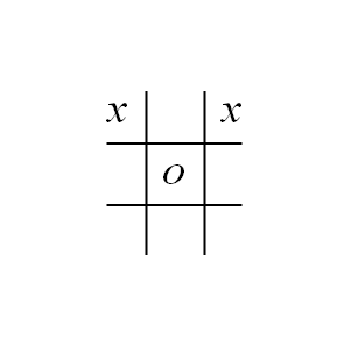
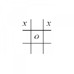
So, for example, the position below would be scored as
2 (for the upper left corner x) + 2 (for the other corner) + 1 (for the top row) = 5.
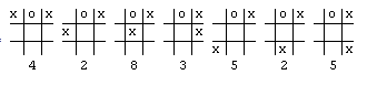
Now, in order to decide on a move, we could just look at every possible move, rate each of the resulting boards, and choose the board with the highest rating. If our tic-tac-toe position was the one below and we were the x player,
then we would have six possible moves. Each move could be rated using our board rating system, and the highest rated board with x in the center and a rating of 8 would be chosen.
This approach was first applied to computer game AI by the famous theoretician Claude Shannon in the paper “Programming a Computer for Playing Chess” (1949), but the idea without the computers actually predates Shannon by hundreds of years. For instance, the chess theoretician Giambatista Lolli published “Osservazioni teorico-pratiche sopra il giuoco degli scacchi ossia il Giuoco degli Scacchi” in 1763. He was the first to publish the idea of counting pawns as 1, bishops as 3, knights as 3, rooks as 5, and queens as 9 thereby giving a rating to every board position in chess (well, at least a rating for the pieces). Shannon modified this rating by subtracting 0.5 for each “doubled” pawn, 0.5 for each “isolated” pawn, 0.5 for each “backward” pawn, and adding 0.1 for each possible move. Thus, if the pieces were the same for both players, no captures were possible, and if the pawns were distributed over the board in a normal fashion, Shannon’s chess AI would choose the move which created the most new moves for itself and removed the most moves from his opponent.
Shannon significantly improved on the idea of an evaluation function by looking more than one move ahead. In two players games, the main algorithm for looking a few moves ahead before applying the evaluation function is the alpha-beta search method which will be tested in a later post.
Let’s try to find and test a few evaluation functions for 2048.
Perhaps the simplest idea for evaluating a position is related to flying. According the great philosopher Douglas Adams,
“There is an art to flying, or rather a knack. Its knack lies in learning to throw yourself at the ground and miss. … Clearly, it is this second part, the missing, that presents the difficulties.” (HG2G).
Suffice it to say that in 2048, the longer you delay the end of the game (hitting the ground), the higher your score (the longer your flight). The game ends when all of the squares are filled with numbers, so if we just count every empty square as +1, then the board rating must be zero at the end of the game.
I ran 1000 simulated games with the Empty Tile evaluation function and got an average ending tile total of 390. The strategy ended the games with a maximum tile of 512 tile 25 times, a 256 tile 388 times, 128 491 times, 64 92 times, and 32 4 times.
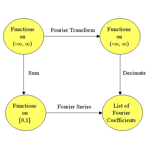
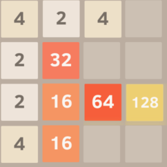
Well, that didn’t seem like anything spectacular. Let’s try to group like tiles—if there are two 128 tiles, let’s try to put them side-by-side. Of course, the idea of putting like tiles together is obvious. Slightly less obvious is the idea of trying to put nearly equal tiles together. Over at stackoverflow.com, the user ovolve, the author of the first 2048 AI, suggested the criteria of “smoothness” in his great post about how his AI worked. There are some interesting ways to measure smoothness with Fourier transforms, but just to keep things simple, let’s measure smoothness by totaling the differences between side-by-side tiles. For example, the smoothness of the board below would be
2+2+4 (first row) + 30+32 (second row) + 14+ 48 + 64 (third row) + 12 + 16 (fourth) + 2+0+2 (first col) + 30+16 + 0 (second) + 4 + 64 + 64 + 128 + 128
which sums to 662.
Once again I ran a 1000 games using smoothness as an evaluation function. The average ending tile total was 720, a new high. The strategy had a maximum ending tile total of 1024 3 times, 512 263 times, 256 642 times, 128 87 times, and 64 5 times. This looks very promising.
Let’s try ovolve’s last criteria — monotonicity. The idea of monotonicity is that we prefer that each row or column is sorted. On the board above, the top row
4 > 2 < 4 > 0 is not sorted. The second 2 < 32 > 0 = 0 and forth 4 < 16 > 0 = 0 rows are sorted only if the spaces are ignored. The third row 2 < 16 < 64 < 128 is fully sorted. Let’s measure the degree of monotonicity by counting how many times we switch from a less than sign to a greater than sign or vice-versa. For the first row we get 2 changes because the greater than sign 4 > 2 changed to a less than sign 2 < 4 and then changed again in 4 > 0. We also get two changes for 2 < 32 > 0, no sign changes in the third row (perfectly monotonic), and two changes in the last row.
I ran 100 games using the monotonicity evaluation function. The average ending tile total was 423. The maximum tile was 512 16 times, 256 325 times, 128 505 times, 64 143 times, and 32 11 times.
I have summarized the results of these three simple evaluation functions in the table below.
Evaluation Func | AETT | Max Tile |
---|---|---|
Empty | 390 | 512 |
Smoothness | 720 | 1024 |
Monotonicity | 420 | 512 |
Cyclic LDRD | 680 | 512 |
Pure Random | 250 | 256 |
Well, clearly Smoothness was the best.
There are three great advantages to numerical evaluation functions over if-then based rules. One, you can easily combine completely different evaluation functions together using things like weighted averages. Two, you can plot the values of evaluation functions as the game proceeds, or even plot the probability of winning against one or two evaluation functions. Three, in 2048, there is the uncertainty where the next random tile will fall. With numerical evaluation functions, we can average together the values of all the possible boards resulting from the random tile to get the “expected value” (or average value) of the evaluation function after the random tile drop.
Well, that’s it for my introduction to evaluation functions. Next time we will focus on more sophisticated evaluation functions and the powerful tree search algorithms that look more than one move ahead.
Have a great day. – Hein
Looks like KUKA Robotics decided to demonstrate the versatility, agility and speed of their Agilus robot by programming it to play ping-pong against a the world-class ping-pong player Timo Boll. Check out the overly dramatic but cool video on Youtube. A few more details can be found at Robohub.
I will be continuing to post articles on AI for the game 2048. The first two articles were:
- An AI for 2048 — Part 1 – which described the game 2048 and reported the results of pure random play and a very simple greedy strategy that just tried to maximize it’s score on every move.
- An AI for 2048 — Part 2 Cyclic Blind Strategies – which reported on strategies that just cyclically repeated the same key stokes.
PROGRAMMING
In this article, I will make some comments on the cyclic blind strategies and report on random blind strategies. The cyclic results can be generated from the Mathematica source code that I posted earlier. The Biased Random results below can be obtained by just modifying the strategy function in the Mathematica source code.
CYCLIC BLIND
In the Cyclic Blind Article, we saw that left-down-right-down had the highest performance of any length 4 or less cyclic strategy with an average end tile total (AETT) of about 680. The other cyclic strategies fell into the following seven groupings:
- All four directions alternating vertical and horizontal (dlur, drul) 420 AETT.
- All four directions without alternating vertical and horizontal (durl, dulr, dlru, …) 270 AETT.
- Three directions with one direction repeated twice in a row where the directions that were not repeated were opposite (durr, dllu, dull, drru, …) 390 AETT
- Three directions with one direction repeated twice in a row where the directions that were not repeated were perpendicular (drrl, duur, ddlu, …) 330 AETT
- Three directions with one direction repeated, but not twice in a row, and the directions that were not repeated were perpendicular (dudr, duru, dldu …) 295 AETT
- Three directions with no repetition (dlu, dur, …) 360 AETT
- One Horizontal Direction + One vertical direction with or without repetition 60 AETT.
BLIND RANDOM BIASED STRATEGIES
The other blind strategy to consider is independent random biased selection of directions. For example, someone might try rolling a six sided die and going left on 1, right on a 2 and down for rolls of 3, 4, 5, or 6. I ran 1000 games each for every possible biased random strategy where the strategy was of the form
left with probability L/T, right with probability R/T, up with probability U/T, down with probability D/T,
where T was the total of L, R, U, and D, and L, R, U and D between 0 and 4.
The results are tabulated below
AETT MAX TILE L/T R/T U/T D/T 11.138 16 1. 0. 0. 0. 55.416 128 0.57 0. 0.43 0. 56.33 128 0.67 0. 0.33 0. 57.17 64 0.5 0. 0.5 0. 57.732 128 0.6 0. 0.4 0. 70.93 16 0.6 0.4 0. 0. 71.246 32 0.57 0.43 0. 0. 71.294 32 0.5 0.5 0. 0. 71.752 32 0.67 0.33 0. 0. 234.42 256 0.4 0.4 0.1 0.1 238.182 256 0.38 0.38 0.12 0.12 241.686 256 0.44 0.33 0.11 0.11 245.49 256 0.44 0.44 0.11 0. 246.148 256 0.4 0.3 0.2 0.1 247.046 256 0.5 0.25 0.12 0.12 247.664 256 0.36 0.36 0.18 0.09 250.372 256 0.43 0.29 0.14 0.14 253.09 256 0.44 0.22 0.22 0.11 254.002 512 0.5 0.38 0.12 0. 255.178 256 0.33 0.33 0.22 0.11 255.242 256 0.33 0.33 0.17 0.17 255.752 256 0.33 0.33 0.25 0.08 257.468 512 0.43 0.43 0.14 0. 258.662 512 0.36 0.27 0.27 0.09 258.832 256 0.57 0.29 0.14 0. 258.9 256 0.36 0.27 0.18 0.18 260.052 256 0.3 0.3 0.2 0.2 261.676 256 0.38 0.25 0.25 0.12 261.902 256 0.31 0.31 0.23 0.15 262.414 256 0.27 0.27 0.27 0.18 263.702 256 0.27 0.27 0.27 0.2 264.034 256 0.31 0.23 0.23 0.23 264.17 512 0.57 0.14 0.14 0.14 264.2 256 0.29 0.29 0.29 0.14 264.226 256 0.31 0.23 0.31 0.15 264.232 256 0.29 0.29 0.21 0.21 264.33 256 0.5 0.17 0.17 0.17 265.328 256 0.33 0.22 0.22 0.22 265.512 256 0.4 0.2 0.3 0.1 265.724 256 0.4 0.2 0.2 0.2 265.918 512 0.33 0.25 0.25 0.17 265.986 256 0.3 0.3 0.3 0.1 266.61 256 0.25 0.25 0.25 0.25 266.796 256 0.29 0.21 0.29 0.21 266.812 256 0.31 0.31 0.31 0.08 267.096 256 0.33 0.17 0.33 0.17 267.5 512 0.33 0.25 0.33 0.08 267.804 256 0.36 0.18 0.27 0.18 267.99 256 0.3 0.2 0.3 0.2 268.414 512 0.43 0.14 0.29 0.14 268.634 256 0.44 0.11 0.33 0.11 271.202 256 0.38 0.12 0.38 0.12 271.646 256 0.33 0.22 0.33 0.11 271.676 512 0.5 0.33 0.17 0. 272.128 256 0.36 0.18 0.36 0.09 273.632 256 0.5 0.12 0.25 0.12 279.82 256 0.4 0.1 0.4 0.1 281.958 256 0.4 0.4 0.2 0. 291.702 512 0.44 0.33 0.22 0. 306.404 256 0.38 0.38 0.25 0. 306.508 512 0.5 0.25 0.25 0. 310.588 512 0.43 0.29 0.29 0. 310.596 512 0.36 0.36 0.27 0. 321.016 512 0.4 0.3 0.3 0. 333.788 512 0.33 0.33 0.33 0. 340.574 512 0.5 0.17 0.33 0. 341.238 512 0.57 0.14 0.29 0. 342.318 512 0.44 0.22 0.33 0. 347.778 512 0.36 0.27 0.36 0. 355.194 512 0.38 0.25 0.38 0. 366.72 512 0.5 0.12 0.38 0. 369.35 512 0.43 0.14 0.43 0. 371.63 512 0.4 0.2 0.4 0. 384.962 512 0.44 0.11 0.44 0.
There are a few things you might notice.
- The best strategy was 44% Left, 11% Right, and 44% down with a AETT of 385 which was much better than pure random (25% in each direction), but not nearly as good as the cyclic strategy left-down-right-down (AETT 686).
- The AETT varies smoothly with small changes in the strategy. This is not surprising. You would think that 55% up, 45% down would have nearly the same result as 56% up and 44% down. The Extreme value theorem then tells us that there must be a best possible random biased strategy.
- The top 17 strategies in the table prohibit one direction with AETTs of 280 to 385.
- If the strategy uses just two directions, then it does very poorly.
Well that’s it for blind strategies. Over the next few posts, we will introduce evaluation functions, null moves, quiescent search, alpha-beta prunning, and expectimax search.