Artificial Intelligence Blog

A proof of Griffin’s Blackjack Theorem

April 17, 2021 in Games, Math by hundalhh | Permalink

Professor Peter Griffin discovered a nice theorem about the best way to count cards in Blackjack. (See the appendix in his book “Theory of Blackjack”). In this note, we review the theorem and reproduce his proof with more detail.

Suppose that you have a wagering game like blackjack which is played with a deck of cards. If you remove some cards from the deck, then the expected value of the game changes. Griffin found an easy formula for estimating the change in expectation caused by the removal of the cards. His formula depends on $E_j$ which is the change in expectation of the game when removing only the $j$th card from the deck.

Assume that the game never requires more than $k$ cards and the deck has $n$ cards in it. Obviously $n\geq k>0$. There are $m = {n \choose k}$ subsets of the deck $I_1, I_2, \ldots, I_m$ that contain $k$ cards each. Let $y_i$ be the expected value of the game played with the card subset $I_i$. We would like to estimate $y_i$ based on the cards in $I_i$.

We can create a linear estimate of $y_i$ by creating a vector $b=(b_1, b_2, \ldots, b_n)$ where $b_j$ is the “value” of the $j$th card. More specifically,
$$
y_i \approx \sum_{j\in I_i} b_j.
$$
Griffin found that the correct formula for $b_j$ is simply $$b_j = (\mu – (n-1) E_j)/k$$ where $\mu$ is the expected value of the game with a fresh deck. Using this value vector $b$ minimizes the squared error of the estimator. This formula is remarkable both for its simplicity and the fact that $k$ only plays a small roll in the calculation.

Griffin’s Theorem Let the error function $e:R^m \rightarrow R$ be defined as

$$
e(b) = \sum_{i=1}^m \left( y_i – \sum_{j\in I_i} b_j \right)^2 .
$$
Then $e(b^*) = \min_{b\in R^m} e(b)$ is the unique global minimum of $e$ where
$$
b^*_j = (\mu – (n-1) E_j)/k
$$
and $\mu$ is the expected value of the game with a fresh deck.

In the theorem above, $e$ is the sum of the squared errors in the linear estimate of the expected value of the game. In order to prove the theorem, we need two lemmas.

Lemma 1 If $\tilde{y}_j$ is the average expectation of the $k$ card subsets that do not contain card $j$, $\bar{y}_j$ is the average expectation of the $k$ card subsets that contain card $j$, and $\mu$ is the expectation of the game with a fresh deck, then
$$\mu = \frac{k}{n}\; \bar{y}_j + \left(1- \frac{k}{n}\right)\tilde{y}_j$$
and
$$\bar{y}_j = \frac{n \mu – (n-k) \tilde{y}_j}{k}.$$

The short proof of this lemma is left to the reader.

Lemma 2
Suppose for $j = 1,\ldots, n$,
$$(2.1)\quad b_j + \alpha \sum_{i=1}^n b_i = \gamma_j.$$ Then

$$ b_j = \gamma_j – \frac{\alpha\; n\; \bar\gamma}{1 + n \alpha}$$
where $\bar\gamma = \frac1n \sum_{j=1}^n \gamma_j$.

Proof: Sum both sides of equation (2.1) to get
$$
n \bar{b} + \alpha n^2 \bar{b} = n \bar{\gamma}
$$
where $\bar{b} = \frac1n \sum_{j=1}^n b_j$. Then,
$$
\begin{aligned}
\bar{b} + \alpha n \bar{b} &= \bar{\gamma} \\
\bar{b} &= \frac{\bar{\gamma}}{1+ n \alpha}.
\end{aligned}
$$
Applying that to equation (2.1) yields
$$
\begin{aligned}
b_j + \alpha \sum_{j=1}^n b_j &= \gamma_j \\
b_j + \alpha n \bar{b} &= \gamma_j\\
b_j + \alpha n \frac{\bar{\gamma}}{1+n \alpha} &= \gamma_j\\
b_j &= \gamma_j – \frac{\alpha\; n\; \bar{\gamma}}{1+n \alpha} \\
\end{aligned}
$$
which completes the proof of the Lemma.

Now we can prove Griffin’s Theorem.

Proof: Let the matrix $X$ be defined by $X_{ij} = 1$ if card $j$ is in set $I_i$ and $X_{ij}=0$ otherwise. We wish to minimize the sum of the squared errors. If we assume that the value of the $j$th card is $b_j$, then we can estimate the expectation of the game played using only card subset $I_i$ with
$$
\sum_{j\in I_i} b_j.
$$
The error of this estimate is $(y_i – \sum_{j\in I_i} b_j)$. The sum of the squared error is
$$
e(b) = \sum_{i=1}^m \left( y_i – \sum_{j\in I_i} b_j \right)^2.
$$
Noice that $\sum_{j\in I_i} b_j = x_i \cdot b$ where $x_i$ is the $ith$ row of $X$. So,
$$
e(b) = \sum_{i=1}^m \left( y_i – \sum_{j=1}^n X_{ij} b_j \right)^2 = \| X b – y \|^2.
$$
In other words $e(b)$ is the square of the distance between $y$ and $Xb$. The Gauss-Markov theorem provides a nice solution for the $b$ which minimizes this distance
$$
b^* = \left(X^T X\right)^{-1} X^T y
$$
where $X^T$ indicates the transpose of $X$. Hence,
$$
(1)\quad X^T X b^* = X^T y.
$$
Let $C=X^T X$. It turns out that $C$ has a very simple structure.

$C_{ij} = x_i^T x_j$ where $x_i$ and $x_j$ are the $i$th and $j$th columns of $X$, so
$$
(2) \quad C_{ii} = x_i^T x_i = { n-1 \choose k-1},
$$
and if $i \neq j$,
$$
(3)\quad C_{ij} = x_i^T x_j = { n-2 \choose k-2}.
$$

So, applying equations (2) and (3) to $i$th row of matrix equation (1) gives

$${n-1 \choose k-1} b_i^* + {n-2 \choose k-2} \sum_{j\neq i} b_j^* = {n-1 \choose k-1} {\bar{y}_i}$$
for $j=1, 2, \ldots n$ where $\bar{y}_j$ is the average expectation of the ${n-1\choose k-1}$ subsets with $k$ cards that contain card $j$.

Note that $$ {n-2 \choose k-2} / {n-1 \choose k-1} = \frac{k-1}{n-1} ,$$ so
$$
\begin{aligned}
b_i^* + \frac{k-1}{n-1} \sum_{j\neq i}^n b_j^* &= \bar{y}_i \\
b_i^* – \frac{k-1}{n-1} b_i^* + \frac{k-1}{n-1} \sum_{j=1}^n b_j^* &=\bar{y}_i \\
\frac{n-k}{n-1} b_i^* + \frac{k-1}{n-1} \sum_{j=1}^n b_j^* &= \bar{y}_i \\
(n-k) b_i^* + (k-1) \sum_{j=1}^n b_j^* &= (n-1) \bar{y}_i\\
b_i^* + \frac{k-1}{n-k} \sum_{j=1}^n b_j^* &= \frac{n-1}{n-k}\bar{y}_i.
\end{aligned}
$$
We apply Lemma 2 with $\alpha = \frac{k-1}{n-k}$ and $\gamma_j = \frac{n-1}{n-k} \bar{y}_j$ to get
$$
\begin{aligned}
b_j^* &= \gamma_j – \frac{\alpha\; n\; \bar\gamma}{1 + n \alpha} \\
&= \frac{n-1}{n-k} \bar{y}_j\; – \frac{\frac{k-1}{n-k}\; n\; \bar\gamma}{1 + n\; \frac{k-1}{n-k}} \\
&= \frac{n-1}{n-k} \bar{y}_j\; – \frac{(k-1) \; n\; \bar\gamma}{n-k + n(k-1)} \\
&= \frac{n-1}{n-k} \bar{y}_j\; – \frac{(k-1) \; n\; \bar\gamma}{n-k + n k-n} \\
&= \frac{n-1}{n-k} \bar{y}_j\; – \frac{(k-1) \; n\; \bar\gamma}{-k + n k} \\
&= \frac{n-1}{n-k} \bar{y}_j\; – \frac{(k-1) \; n\; \bar\gamma}{k (n-1)} \\
&= \frac{n-1}{n-k} \bar{y}_j\; – \frac{(k-1) \; n\; \frac{n-1}{n-k} \mu }{k (n-1)} \\
&= \frac{n-1}{n-k} \bar{y}_j\; – \frac{(k-1) \; n\; \mu }{(n-k)k}. \\
\end{aligned}
$$
By Lemma 1,
$$\bar{y}_j = \frac{n \mu – (n-k) \tilde{y}_j}{k},$$
so
$$
\begin{aligned}
b_j^*
&= \frac{n \mu – (n-k) \tilde{y}_j}{k} \frac{n-1}{n-k} – \frac{ n (k-1)\mu}{k (n-k)} \\
&= \frac{ n (n-1) \mu }{(n-k)k} – \frac{ (n-k) \tilde{y}_j (n-1)}{k(n-k)} – \frac{ n (k-1)\mu}{k (n-k)} \\
&= \frac{ n (n-1) \mu }{(n-k)k} – \frac{ n (k-1)\mu}{k (n-k)} – \frac{ (n-k) \tilde{y}_j (n-1)}{k(n-k)} \\
&= \frac{n \mu}{k} \left[ \frac{n-1}{n-k} - \frac{k-1}{n-k} \right] – \frac{ \tilde{y}_j (n-1)}{k} \\
&= \frac{n \mu}{k} – \frac{ \tilde{y}_j (n-1)}{k} \\
&= \frac{n \mu – (n-1) \tilde{y}_j}{k} \\
&= \frac{\mu – (n-1) (\tilde{y}_j- \mu)}{k} \\
&= \frac{\mu – (n-1) E_j}{ k }
\end{aligned}
$$
which completes the proof.

In the future, I hope to write some articles about how Griffin’s Theorem can be applied to other games.

I should mention that it is not too hard to extend Griffin’s Theorem to get more accurate quadratic approximation of the expectation of the game with card removal (or higher degree polynomial approximations).

Visualizing Cramer’s Rule

March 30, 2021 in Math by hundalhh | Permalink

I posted the comment below on Reddit.

It easy for me to recall the geometric picture Cramer’s rule in my head, but it took an hour or more to write down an explanation.

Suppose that the vector $y = a_1 x_1 + a_2 x_2 + \cdots + a_n x_n$
where $y, x_1, x_2, \ldots, x_n$ are all vectors in $R^n$ and $a_1,a_2, \ldots, a_n$ are real.

(We will assume that $\det(x_1,x_2, \ldots, x_n)$ is not zero.)
For me, Cramer’s rule is just two hyperparallelepiped (squished hypercubes) which share the same base.

The first “parallelepiped” has edges $a_1 x_1, a_2 x_2, a_2 x_3,\ldots, a_nx_n$.
The second “parallelepiped” has edges $y, a_2 x_2, a_2 x_3,\ldots, a_n x_n.$
The shared base has edges $a_2 x_2, a_3 x_3,\ldots, a_n x_n$.

The volume of the first “parallelepiped” is $\det(a_1 x_1, a_2 x_2, \ldots, a_n x_n)$.
The volume of the second “parallelepiped” is $\det(y, a_2 x_2, \ldots, a_n x_n)$.
There are two key insights:

1) these parallelepipeds have the same “height” and base, and hence the same volume.
2) the ratio of the volumes is 1, so

1 = “volume of parallelepiped 1″/”volume of parallelepiped 2″ (by insight 1)
= $\frac{\det(a_1 x_1, a_2 x_2, \ldots, a_n x_n)}{\det(y, a_2 x_2, a_3 x_3, \ldots, a_n x_n)}$
= $a_1 \frac{\det(x_1, x_2, \ldots, x_n)}{\det(y, x_2, x_3, \ldots, x_n)}$ (by linearity of the determinant).

The second insight leads directly to Cramer’s rule by multiplying both sides of the equality by
$$\frac{\det(y, x_2, \ldots, x_n)}{\det(x_1, x_2, x_3, \ldots, x_n)}.$$

Why is the first insight true?

To explain this
let B= span(base) = $span(x_2,x_3, \ldots, x_n)$ and
let A= the one dimensional subspace perpendicular to A.

Think of the surface of a table as being B. The height of each parallelepiped is the distance from B to the points in the parallelepiped which are farthest away from B.
The height of the first cube, $h_1$, is the distance from the base which lies in B to the “top” of the parallelepiped 1 which is parrallel to B.
$$h_1 = proj_A(a_1 x_1) = a_1 proj_A(x_1).$$

The height of the second cube, $h_2$, is the distance from the base which lies in B to “top” of the parallelepiped 2 which is parrallel to B.
$$h_2 = proj_A(y).$$

But, by the defintion of y and the fact that A is perpendicular to $x_2,x_3, \ldots, x_n,$
$$
\begin{aligned}
h_2 &= proj_A(y)\\
&= proj_A(a_1 x_1+a_2 x_2+\cdots+a_n x_n) \\
&= proj_A(a_1 x_1) + proj_A(a_2 x_2+\cdots+a_n x_n) \\
&= proj_A(a_1 x_1) \\
&= a_1 proj(x_1) \\
&= h_1.
\end{aligned}
$$
This shows that the “heights of the two parallellepipeds are equal, so the volumes must be equal because they share the same base.

———————————————

Here is almost same idea with a lot fewer words.
Assume without loss of generality that the space is $span(x_1,x_2, \ldots, x_n)$

Let B = $span( x_2, x_3, \ldots, x_n)$.
Let A = the 1 dimensional subspace which is perpendicular to A.
Then
$$
\begin{aligned}
proj_A y &= proj_A (a_1 x_1+ \cdots + a_n x_n) \\
&= proj_A (a_1 x_1) \\
&\mathrm{\ \ \ \ (due\ to\ linearity\ and\ the\ fact\ that\ B\ is\ perpendicular\ to\ } x_2,x_3,\ldots, \mathrm{\ and\ } x_n)\\
&= a_1 proj_A(x_1).
\end{aligned}
$$

So, $|a_1| = \frac{length( proj_A\; y)}{ length( proj_A\; x_1)}.$

Let
$\alpha = |\det(x_1,x_2,\ldots, x_n)|$ = “volume of the parallelepiped with edges $x_1, x_2, x_3, \ldots, x_n$”,
$\beta = |\det(y, x_2,\ldots, x_n)|$ = “volume of the parallelepiped with edges $y, x_2, x_3, \ldots, x_n$”, and
$\gamma =$ “area of the hyperrhombus with edges $x_2, x_3, \ldots, x_n$”.

$\alpha = length( proj_A x_1)\; \gamma$
$\beta = length( proj_A y)\; \gamma$

Finally,
$$
\begin{aligned}
|a_1| &= \frac{length( proj_A y) }{ length( proj_A x_1)} \\
&= \frac{|length( proj_A y) \gamma| }{ | length( proj_A x_1) \gamma) |} \\
&=\frac{ |\det(y, x_2, \ldots, x_n)| }{ |\det(x_1, x_2, \ldots x_n)|}.
\end{aligned}
$$

A Simple Minesweeper Puzzle

February 8, 2021 in Games, Logic, Statistics by hundalhh | Permalink

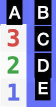
Suppose that you are playing the game Minesweeper. On your first move, you click on the lower left corner square and reveal a 1. Then you click on the square above the corner and reveal a 2. Then you click on the square above that and reveal a 3. What is the “safest” next move?

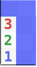
In order to talk about the contents of the blue squares, we will label them A,B,C,D, and E.

There are only three possible scenarios:

a) A, B, C, and E have mines,

b) A, C, and D have mines, or

c) B, C, and D have mines.

But, not all of these scenarios are equally likely. Suppose there are a total of $m$ mines on the board and $s$ squares left excluding the eight that we are looking at. Then the total number of possible distributions of the mines for scenarios a, b, and c are:

$n_a = {s\choose m-4},$
$n_b= {s\choose m-3},$ and
$n_c ={s\choose m-3}.$

These scenarios are not equally likely. (Above we used choose notation. ${n\choose m}= \frac{n!}{m! (n-m)!}$ where $n!=1\cdot2\cdot3\cdot\cdots\cdot n$. For example 4!=24 and ${5\choose 2}=\frac{5!}{2!\ \cdot\ 3!} = \frac{120}{2 \cdot 6}= 10$.) In fact,

$$\begin{aligned} r=\frac{n_b}{n_a}&=\frac{s\choose m-3}{s\choose m-4} \\&=\frac{\frac{s!}{(m-3)! (s-(m-3))!}}{\frac{s!}{(m-4)! (s-(m-4))!}}\\&=\frac{\frac{1}{(m-3)! (s-(m-3))!}}{\frac{1}{(m-4)! (s-(m-4))!}}\\&= \frac{(m-4)! (s-(m-4))!}{(m-3)! (s-(m-3))!}\\&= \frac{ (s-m+4)!}{(m-3) (s-m+3))!}\\&= \frac{ s-m+4}{m-3 }.\end{aligned}$$

In the beginning of the game $r\approx s/m-1\approx 4$, so scenarios b and c are about four times as likely as scenario a. We can now estimate the probabilities of scenarios a, b, and c to be about

“probability of scenario a” = $p_a \approx 1/9,$
“probability of scenario b” = $p_b \approx 4/9, and$
“probability of scenario c” = $p_c \approx 4/9.$

We can now conclude that the probability that square A has a mine is 5/9, that square B has a mine is 5/9, that square C has a mine is 100%, that square D has a mine is 8/9, and that square E has a mine is 1/9, so square E is the “safest” move.

Generally speaking, scenarios with more mines are less likely if less than half of the unknown squares have mines.

Another interesting way to think about it is that the 3 and 2 squares pulled the mines toward them making square E less likely to contain a mine.

You can approximate the probability of each scenario by just assuming that the squares are independent random variables (a false, but almost true assumption) each of which has probability $m/s$ of containing a mine. Using that method gives the same results as the approximation above.

If you prefer an exact calculation, then use the formula

$$ r=\frac{ s-m+4}{m-3 }$$

to get the exact ratio of $\frac{p_b}{p_a} = \frac{p_c}{p_a}=r$.

(PS: Jennifer told me via email that you can play Minesweeper online at https://www.solitaireparadise.com/games_list/minesweeper.htm)

A very basic description of the binomial distribution

February 7, 2021 in Statistics by hundalhh | Permalink

I wrote this up for a friend this morning. Hopefully someone else can benefit from it.

Part 1 – The relationship between the expansion of (x+y)^n and the binomial distribution

The binomial distribution for n coin flips and i heads is the probability of getting i heads with n independent coin flips assuming the probability of getting one head with one coin toss is p. (In the explanations below, we will always assume that the coin flips are independent.)

There is a very strong relationship between the binomial distribution and the expansion of (x+y)^n.

For example, for n=1 if we set x=1/3 and y=2/3, then

(x+y)^1 = x+ y = 1/3 + 2/3.

If a person flips a biased coin once and the probability of heads is 1/3, then the two possible outcomes are

– one head with probability 1/3, or

– one tail with probability 2/3.

For n=2 if we set x=1/3 and y=2/3, then

(x+y)^2

= (x+ y)*(x+y)

= x*(x+y) + y*(x+y)

= x*x + x*y + y*x + y*y

= x^2 + 2*x*y + y^2

= (1/3)^2 + 2*(1/3)*(2/3) + (2/3)^2.

(I am using * to indicate multiplication which is common for programmers. Mathematicians tend to omit the * and write x y to indicate x times y.)

If a person flips a biased coin twice and the probability of each heads is 1/3, then there are the following possible outcomes:

– two heads HH with probability (1/3)^2,

– one head and tail, HT or TH 2*(1/3)*(2/3), or

– two tails TT with probability (2/3)^2.

For n=3 if we set x=1/3 and y=2/3, then

(x+y)^3

= (x+y)*(x+y)^2

= (x+y)*(x*x + x*y +y*x + y*y)

= x*(x*x + x*y +y*x + y*y) + y*(x*x + x*y +y*x + y*y)

= x*x*x + x*x*y + x*y*x + x*y*y + y*x*x + y*x*y + y*y*x + y*y*y

= x^3 + 3*x^2*y + 3*x*y^2 + y^3

= (1/3)^3 + 3*(1/3)^2*(2/3)^2 + 3*(1/3)*(2/3)^2 + (2/3)^3.

If a person flips a biased coin three times and the probability of heads is 1/3, then there are the following possible outcomes:

– three Heads HHH with probability (1/3)^3,

– two heads and one tail, HHT, HTH, THH with probability 3*(1/3)^2*(2/3),

– one head and two tails, HTT, THT, TTH with probability 3*(1/3)*(2/3)^2, or

– three tails TTT with probability (2/3)^3.

Notice that every possible sequence of H’s and T’s for 3 flips can be obtained by fully expanding (x+y)^3 and replacing the x’s and y’s with H’s and T’s. This shows that there is a very strong correspondence between the results of n coin flips and the expansion of (x+y)^n. Note also that ( 1/3 + 2/3)^n = 1^n = 1, so all these probabilities will add up to 1.

Part 2 -Pascal’s Triangle

If we look more closely at the expansion of (x+y)^n, we see a pattern.

(x+y)^0 = 1

(x+y)^1 = 1*x+1*y

(x+y)^2 = 1*x^2 + 2*x*y + 1*y^2

(x+y)^3 = 1*x^3 + 3*x^2*y + 3*x*y^2 +1* y^3

(x+y)^4 = 1*x^4 + 4*x^3*y + 6*x^2*y^2+ 4*x*y^3 + 1*y^4

(x+y)^5 = 1*x^5 + 5*x^4*y + 10*x^3*y^2+ 10*x^2*y^3 + 5*x*y^4 + 1*y^5.

…

Looking just at the numbers in each expansion gives us a triangle which is knows as Pascal’s triangle:

1 1

1 2 1

1 3 3 1

1 4 6 4 1

1 5 10 10 5 1

1 6 15 20 15 6 1

Every number is the sum of the two numbers “above” it. These numbers can be obtained from the formula

(n choose i) = n!/ ( i! * (n-i)!)

where n is the row number and i=0,1,2,…, n.

For example, in the 5th row the third entry corresponds to i=2.

b(5,1) = 5!/( 2! * 3!) = 120/( 2 * 6) = 120/12=10.

Where does the formula for (n choose i) come from? It comes from the fact that there are exactly n! ways to order the numbers 1,2,3, …, n. For example, for n=5, there are 5!=120 ways to order the numbers 1,2,3, 4, and 5.

12345 12354 12435 12453 12534 12543 13245 13254 13425 13452 13524

13542 14235 14253 14325 14352 14523 14532 15234 15243 15324 15342

15423 15432 21345 21354 21435 21453 21534 21543 23145 23154 23415

23451 23514 23541 24135 24153 24315 24351 24513 24531 25134 25143

25314 25341 25413 25431 31245 31254 31425 31452 31524 31542 32145

32154 32415 32451 32514 32541 34125 34152 34215 34251 34512 34521

35124 35142 35214 35241 35412 35421 41235 41253 41325 41352 41523

41532 42135 42153 42315 42351 42513 42531 43125 43152 43215 43251

43512 43521 45123 45132 45213 45231 45312 45321 51234 51243 51324

51342 51423 51432 52134 52143 52314 52341 52413 52431 53124 53142

53214 53241 53412 53421 54123 54132 54213 54231 54312 54321

We could call these 120 orderings.

If we look at the first two numbers in every 5 digit ordering above, there are only 10 possible prefixes: 12, 13, 14, 15, 23, 24, 25, 34, 35, and 45. So there are 10 ways to choose two numbers from a list 1,2,3,4, 5. Mathematicians would say that

(5 choose 2) = 10.

After you choose 2 numbers, there are 3 remaining. We can get every one of the 120 ordering by

a) taking each of the 10 choices of 2 numbers from 5,

b) looking at how many ways each of the chose numbers can be ordered. In this case the chosen can be ordered 2!=2 ways. (For example, 13 could ordered as 13 or 31.), and

c) looking at how many ways the unchosen numbers can be ordered. In this case each choice can be ordered 3!=6 ways. (For example, if we chose 13, then 2, 4, and 5 remain and those numbers can be ordered as 245, 254, 425, 452, 524, and 542.)

So there were 2! orderings for the first 2 and 3! orderings for the remaining 3. All 120 orderings can be found by

a) one of 10 choices, (10 = 5 choose 2),

b) one of the 2 ways to order the chosen, (2=2!) and

c) one of the 6 ways to order the unchosen (6=3!).

The resulting formula is

Number of orderings of 1,2,3,4, and 5 = 5! = 120 = 10*2*6 = (5 choose 2)*2!*3!.

In general, if you have the numbers 1,2,…, n, and you choose i numbers, then every one of the n! orderings can be reproduced from

a) (n choose i) ways to select i numbers from the list 1,2,3,…,n,

b) i! ways to order the i chosen numbers, and

c) (n-i)! ways to order the unchosen.

The resulting formula is

n! = (n choose i) * i! * (n-i)! .

If we divide both sides by i! * (n-i)!, we get

n! / ( i! * (n-i)! ) = (n choose i).

Part 3 – Conclusion

We showed that there is a very strong relationship between the expansion of (x+y)^n and the binomial distribution of n coin flips. The coefficient for each term of (x+y)^n has the formula

(n choose i) = n!/( i! * (n-i)! ).

We derived this formula. The final result is that the probability of getting i heads when flipping n coins each of which has probability p of heads is

“the number of ways of choosing which of the n coins are heads” * “the probability of flipping i heads in a row” * “ the probability of flipping (n-i) tails in a row”

= (n choose i) * p^i * (1-p)^(n-i)

= n!.( i! * (n-i)! ) * p^i * (1-p)^(n-i).

Some Notes on Optimal Portfolio Theory

February 5, 2021 in Investing, Optimization by hundalhh | Permalink

This note just reviews the derivation of portfolios that maximize the Sharpe ratio.

Suppose that you have some stocks that you want to invest in. We will think of the returns of these stocks as being a random column vector $G$ in $R^n$. Suppose that $r=E[G]\in R^n$ is a vector of the expected return of the stocks and $C= E\left[ (G-r) (G-r)^T\right]$ is the covariance matrix of $G$ with the superscript $T$ indicating the transpose, thus $C\in R^{n\times n}$.

We will often want to maximize the Sharp ratio of a portfolio which is defined as the expected return of the portfolio minus the risk free return divided by the standard deviation. In order to simplify the math a little, we will assume that the risk free return is 0 and $C$ is positive definite, $a^T C a>0$ for all vectors $a\in R^n\setminus\{0\}$. Thus for our purposes, the Sharpe ratio for an “allocation vector” $a\in R^n\setminus\{0\}$ will be defined $$\rho(a) := \frac{E[a^T G]}{\sqrt{E[ (a^T G - a^T r)^2]}} = \frac{a^T r}{\sqrt{a^T C a}}.$$ We could say that the allocation vector is in dollars, so $a_1$ would be the dollar value of the stocks held in the portfolio for the first stock. The value of $a_1$ could be negative indicating that the stock was shorted.

It is helpful to notice that the Sharpe ratio does not change if we double or triple the amount invested in each stock. In fact, for any real number $\gamma\neq 0$ and any nonzero allocation vector $a\in R^n$, $$\rho(\gamma a)= \gamma \rho(a).$$ So, when maximizing $\rho$ we can restrict ourselves to vectors $a$ where $a^T C a=1$.

The matrix $C$ is real symmetric positive semidefinite, so it has a Cholesky decomposition $C=U^T U$ where $U$ is upper triangular. Let $u= U a$. Then $$1=a^T C a= a^T U^T U a = u^T u= ||u||^2, $$ so $u$ has norm 1. Thus if we want to maximize $\rho(a)$, it suffices (by restricting to vectors $a$ where $a^T C a=1$) to maximize $$\rho(a) = \frac{a^T r}{\sqrt{a^T C a}} = a^T r = u^T U^{-T} r$$ over all unit vectors $u$. (We use $U^{-T}$ to denote $(U^T)^{-1}$, the inverse transpose of $U$.) The unit vector which maximizes $u^T U^{-T} r$ is simply $$u^*= \frac{U^{-T} r}{|| U^{-T} r||}.$$ We can now generate an optimal allocation vector $a^*$ by

$$ a^* = U^{-1} u^*= \frac{U^{-1} U^{-T} r}{|| U^{-T} r||} = \frac{ (U^T U )^{-1} r}{|| U^{-T} r||} = \frac{ C^{-1} r}{|| U^{-T} r||}.$$ The scalar factor $|| U^{-T} r||$ has no effect on $\rho$, so $$a^{**} = C^{-1} r$$ is also an optimal allocation vector. Note that the Sharpe ratio of $a^*$

$$\rho(a^{**})=\rho(a^*)=\frac{(a^{*})^T r}{\sqrt{(a^{*})^T C a^*}}=(a^{*})^T r= \frac{r^T U^{-1} U^{-T} r}{|| U^{-T} r||}= || U^{-T} r||.$$

Example 1

Suppose that you want to invest in two uncorrelated stocks. Assume that their expected returns are $r=( 0.001, 0.001)^T$ and their covariance matrix is $$C=\left(\begin{matrix} 10^{-4} & 0 \\ 0 & 10^{-4}\end{matrix}\right).$$ All optimal allocations $a$ of the stocks are multiples of $$a^{**} = C^{-1} r = \left(\begin{matrix} 10^{4} & 0 \\ 0 & 10^{4}\end{matrix}\right)( 0.001, 0.001)^T= (10, \ 10)^T.$$ This merely indicates that the optimal Sharpe ratio is attained if and only if you invest the same amount in money in each of these stocks.

EXAMPLE 2

Suppose that you want to invest in two uncorrelated stocks. Assume that their returns are $r=( 0.001, 0.0005)^T$ and their covariance matrix is $$C=\left(\begin{matrix} 10^{-4} & 0 \\ 0 & 10^{-4}\end{matrix}\right).$$ All optimal allocations $a$ of the stocks are multiples of $$a^{**} = C^{-1} r = \left(\begin{matrix} 10^{4} & 0 \\ 0 & 10^{4}\end{matrix}\right)( 0.001, 0.0005)^T= (10, \ 5)^T.$$ This indicates that the optimal Sharpe ratio is attained if and only if you invest the twice as much money in the first stock and a nonzero amount of money is invested. Note that Kelly Criterion often indicates that your bets should be proportional to the edge of your investments, so it gives similar advice.

EXAMPLE 3

Suppose that we have two gamblers. The first gambler is willing to give you 2.2 times your wager if candidate A wins the election, but you lose the bet if candidate A does not win. (I.e. if you wager $\$10$ with the first gambler, the your net gain will be $\$22 – \$10 = \$12$ if you win.) The second gambler is willing to pay you twice your bet if candidate B wins and you lose your bet with the second gambler if candidate B loses.

This could be called an arbitrage situation.

Let’s assume that there is a 50% chance that candidate A will win and a 50% chance that candidate B will win. We can think of each gambler as being a stock that we can invest in. The expected value of the first gambler is 0.1 (i.e. if you wager ${\$}10$ with the first gambler, your expected net gain is 0.1*${\$}10$ = ${\$}1$.) The expected value of the second gambler is 0. The covariance matrix requires some computations.

$$C_{11} = E[ (G_1-r_1)^2] = 1/2 ( (1.2 – 0.1)^2 + (-1 – 0.1)^2 ) = 1.21.$$

$$C_{12} = C_{21} = E[ (G_1-r_1)(G_2-r_2)] = 1/2 ( (1.2 – 0.1)(-1) + (-1 – 0.1)1 ) = -1.1.$$

$$C_{22} = C_{21} = E[ (G_2-r_2)^2] = 1/2 ( (-1)^2 + (1)^2 ) = 1.$$ $$C = \left(\begin{matrix} 1.21 & -1.1 \\ -1.1 & 1 \end{matrix}\right).$$

Interestingly, $C$ is not invertible. This is because $(10, 11) C (10, 11)^T = 0$. This means that if you wager $\$10$ with gambler 1 and $\$11$ with gambler 2, you will always win $\$1$. If candidate A wins, then you gain $\$12$ from the first gambler and lose $\$11$ to the second. If candidate B wins, then you lose $\$10$ to the first gambler and gain $\$11$ from the second. Since you always win $\$1$, your volatility is zero and your Sharpe ratio is infinite. In the derivation, we assumed that $C$ was positive definite, but in this example, it is not.

In a future post, I would like to give a few more examples and maybe even compare the optimal Sharp ratio allocation with a Kelly allocation.

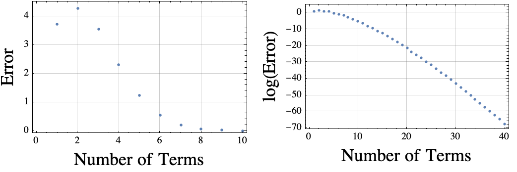
One reason why I want 30 digits of Pi or even more

January 25, 2021 in Math by hundalhh | Permalink

I was wondering how fast the Taylor Series for $\exp(\pi i)$ would converge. According to Taylor,

$$\exp(\pi i) = 1 + (\pi i) + (\pi i)^2/2! + (\pi i)^3/3! + (\pi i)^4/4! + \ldots = \sum_{j=0}^\infty \frac{(\pi i)^j}{j!}.$$

According to Euler, $\exp(\pi i)= -1$. I wanted to estimate the convergence rate, so I just fired up Mathematica and plotted the values of $$error(k) = \left| 1+ \sum_{j=0}^k \frac{(\pi i)^j}{j!}\right|.$$ The Mathematica plot is shown below.

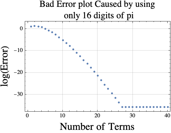
It occurred to me that Mathematica knows thousands of digits of pi. I could force it to only use the first 16 digits by using double precision floating point numbers. If I do that, then the log(Error) plot is “wrong” because the approximation for pi is not accurate enough. The erroneous plot is shown below.

If you want a good estimate of the truncated Taylor series error using $k$ terms, you could use the absolute value of term $k+1$ which is

$$error(k)\approx f(k)= \frac{\pi^{k+1}}{(k+1)!}$$.

Here is a plot of $r(k)= error(k)/f(k)$. If the estimator is good, then the $r(k)$ values (y-coordinates) should be near 1.

Creating these plots requires around 30 digits of pi! If I wanted to look at more terms, I would need more digits of pi.

Here is the code I used to generate the plots.

SetOptions[ListPlot, GridLines -> Automatic, Frame -> True, ImageSize -> 250];
error[k_] := Abs[ 1 + Sum[ (I Pi)^j/j!, {j, 0, k}]];
plt0 = ListPlot[ Array[error, 10], Frame -> True, 
 FrameLabel -> (Style[#, 18] & /@ {"Number of Terms", "Error"})];
plt1 = ListPlot[Log[ Array[error, 40]],
 FrameLabel -> (Style[#, 18] & /@ {"Number of Terms", 
 "log(Error)"})];
error[k_] := Abs[ 1 + Sum[ (I N[Pi])^j/j!, {j, 0, k}]];
plt3 = ListPlot[Log[ Array[error, 40]], Frame -> True, 
 FrameLabel -> (Style[#, 18] & /@ {"Number of Terms", "log(Error)", 
 "Bad Error plot Caused by using only 16 digits of pi", " "}), 
 PlotLabel -> 
 Style["Bad Error plot Caused by using\n only 16 digits of pi", 
 16]];
errorRat[k_] := 
 Abs[ 1 + Sum[ (I Pi)^j/j!, {j, 0, k}]]/ (Pi^(k + 1)/(k + 1)! );
plt4 = ListPlot[Array[errorRat, 40], Frame -> True, 
 FrameLabel -> (Style[#, 18] & /@ {"Number of Terms", 
 "error(k)/f(k)"}), 
 PlotLabel -> 
 Style["Plot error(k) divided by estimated\n error(k) for \
k=1,2,..., 40", 16]];

Maximizing a function over integers (Part 3)

December 31, 2020 in Math by hundalhh | Permalink

In part 1, we defined the term strictly concave and introduced the theorem that if $f$ is strictly concave and $f(x)=f(x+1)$, then the integer(s) that maximize $f$ are exactly the set $\{\mathrm{floor}(x+1), \mathrm{ceil}(x)\}$ which is usually a set containing only one number $\mathrm{round}(x+1/2)$. In part 2, we showed how the theorem in part 1 can be used to prove that the maximum value that can be obtained when putting an integer into $f(x)=a x^2 + b x + c$ is $f(i)$ where $i=\mathrm{round}(-b/(2a))$ (assuming $a<0$).

The next theorem says that the real number $x$ that maximizes $f$ is always near the integer $i$ that maximizes $f$.

THEOREM #3

$f$ is a real valued strictly concave function,
there is a real number $x$ such that $f(x)$ is the maximum value that $f$ attains with real inputs, and
there is an integer $i$ such that $f(i)$ is the maximum value that $f$ attains with integer inputs,

then $|x-i|<1$.

The idea of the proof is fairly simple. Suppose that $i>x+1$. Then $i-1>x$. So $i-1$ is between $i$ and $x$. Concavity implies that that the point $(i-1, f(i-1))$ lies above the line connecting $(x, f(x))$ and $(i,f(i))$, but $f(x)\geq f(i)$.

The fact that the point $(i-1, f(i-1))$ is above the line implies that $f(i-1)> f(i)$, but that contradicts the definition of $i$, so using proof by contradiction, $i\leq x+1$. The other cases are either similar or easy.

EXAMPLE

Find the maximum value of $f(x) = x (x-14) (x-20)$ among all integers between 0 and 14.

Finding the maximum among reals is easy if you know differential calculus and the quadratic formula. According to differential calculus, the maximum can only occur if the “derivative” of $f(x)$ is zero. $$f(x) = x (x-14) (x-20) =x^3-34 x^2 + 280x.$$ The derivative of a polynomial can be found by multiplying the coefficient by the exponent and decreasing the exponent by 1. The result is $$f'(x) = 3 x^2 -68 x + 280.$$ If we put that in the quadratic formula, we get $$x=\frac{68\pm\sqrt{68^2 – 4 \cdot 3 \cdot 280}}{2 \cdot 3} = \frac{68\pm\sqrt{1264}}{6}\approx 5.41\ \mathrm{or\ } 17.26.$$ It turns out that 17.26 is a local minimum, so the local maximum occurs when $x\approx 5.41$. According to the theorem, any integer $i$ that maximizes $f(i)$ must be within 1 of 5.41, so that integer can only be 5 or 6. Now $f(5)= 675$ and $f(6) = 672$, so 5 is the integer that maximizes $f$. Incidentally, $f(5.41) = 678.025021$ and the true maximum of $f(x)$ is $$f\left(\frac{68-\sqrt{1264}}{6}\right) = \frac{16}{27} \left(442+79 \sqrt{79}\right)\approx 678.025101610626.$$

We could actually use the theorem from part 1 to find the integer $i$ that maximizes $f(i)$. Solving $f(x)=f(x+1)$ using the quadratic formula gives $$x=\frac{1}{6} \left(65\pm\sqrt{1261}\right).$$ If you replace the $\pm$ with the plus sign, you get the local minimum. If you replace it with the minus sign, you get $$\frac{1}{6} \left(65-\sqrt{1261}\right)\approx 4.91.$$ According to the theorem from part 1, the integer that maximizes $f(x)$ must be round(4.91+1/2)=round(5.41)=5. Often it is easier to find the maximum of $f$ rather than trying to solve $f(x)=f(x+1)$, so that is why the theorem above is useful.

If you want to see a more formal mathematical writeup, click here. That PDF shows how you can generalize the three given theorems to a larger class of functions that are not necessarily strictly concave. Also, in the last section of the paper, we sharpen the bound on the difference between the real maximum and the integer maximum. Above, we showed that this difference was less than 1. If $f$ is continuously twice differentiable, then sharper bounds can be computed.

This concludes the three part series.

Maximizing a function over integers (Part 2)

December 26, 2020 in Math, Optimization by hundalhh | Permalink

Parabolas

The simplest concave functions are parabolas with the vertex at the top. All parabolas can be described by three real numbers $a$, $b$, and $c$, and the formula $y=a x^2 + b x + c$. For strictly concave parabolas $a<0$. For example, if $a=-2$, $b=3$, and $c=5$, then the function $y= f(x) = -2x^2 + 3 x +5$ is the parabola shown below.

If the vertex (shown above in blue) is above the x-axis, then the x-coordiante of the vertex can be computed by finding the points where the concave parabola crosses the x-axis (shown above in orange). In our case, the parabola $y=f(x)$ crosses the x-axis when $0=y=f(x)$, or when $$\begin{aligned}0&= -2x^2 + 3 x +5\\0&=-(2x^2-3×-5)\\0&=-(2×-5)(x+1).\end{aligned}.$$ If $0=\alpha\cdot \beta$, then either $\alpha=0$ or $\beta=0$. So, the parabola crosses the x-axis when either $0=2×-5$ or $0=x+1$ which means that it crosses when $x=5/2$ or $x=-1$. Parabolas are symmetric about the vertical line going through the vertex, so the x-coordinate of the vertex is half way between the x-coordinates of the crossing points (a.k.a the roots of $f(x)$). $$\begin{aligned} x_\mathrm{vertex} &= \frac{x_\mathrm{crossing1} + x_\mathrm{crossing2}}2\\&= \frac{ -1 +5/2}2\\&=\frac{3/2}2\\&=3/4.\end{aligned}$$

So the x-coordinate of the vertex is $x=3/4$. This is also the real number that maximizes $f(w)$ over all real numbers $w$.

In general, the x-coordinates of the crossing points can be found with the quadratic formula $$x=\frac{-b\pm\sqrt{b^2-4ac}}{2 a}.$$ The $\pm$ sign means that one crossing can be found by replacing $\pm$ with + and the other can be found by replacing the $\pm$ with -. But, if you have one number that is $x_1=\alpha+\beta$ and another that is $x_2=\alpha-\beta$, then the average of the two numbers is just $\alpha$. In other words if the two values of $x$ are $x=\alpha\pm\beta$, then the average value is just $\alpha$. So, to computer the average x-coordinate of the crossing points, all we have to do is remove the $\pm$ sign and whatever it is applied to from the quadratic formula. $$ x_\mathrm{vertex} = \frac{-b}{2 a}.$$

theorem #2

Informally, if $y=f(x)$ is a parabola, $f(x) = a x^2 + b x + c$, and $a<0$, then the integer(s) that maximize $f(x)$ are the set $\{\mathrm{floor}(x+1/2), \mathrm{ceil}(x-1/2)\}$ where $x=\frac{-b}{2 a}$.

If $x$ is an integer plus 1/2 (e.g. 2.5, 7.5, …), this set has two elements $x+1/2$ and $x-1/2$. If $x$ is not an integer plus 1/2, the set has only one element $\mathrm{round}(x)$ and that is the integer that produces the highest possible value of $f(z)$ among all integers $z$.

examples

Example 1: If $f(x)= -2x^2 + 3 x +5$, then $a=-2$, $b=3$, and $c=5$. The values of $x$ in the theorem is the same as the x-coordinate of the vertex $$x=\frac{-b}{2a} = \frac{-3}{2\cdot(-2)}= \frac{-3}{-4}=3/4.$$ The integer(s) that maximize $f(z)$ among all integers $z$ are the set $$\begin{aligned}\{\mathrm{floor}(x+1/2), \mathrm{ceil}(x-1/2)\}&= \{\mathrm{floor}(3/4+1/2), \mathrm{ceil}(3/4-1/2)\}\\&= \{\mathrm{floor}(5/4), \mathrm{ceil}(1/4)\}\\&=\{1\}.\end{aligned}$$

Example 2: If we lower the parabola from example 1 by a little bit setting $f(x)= -2x^2 + 3 x +\sqrt{17}$, then $a=-2$, $b=3$, and $c=\sqrt{17}$. The value of $x$ in the theorem is the same as the x-coordinate of the vertex $x=\frac{-b}{2a} =3/4.$ The result does not depend on $c$, so as in example 1, the integer that maximizes $f(z)$ among all integers $z$ is $z=\mathrm{round}(3/4)=1$.

Example 3: $f(x)= -x^2+x = (1-x)x$, then $a=-1$, $b=1$, and $c=0$. The value of $x$ in the theorem is the same as the x-coordinate of the vertex $$x=\frac{-b}{2a} =\frac{-1}{2\cdot (-1)}=1/2.$$ The integer(s) that maximize $f(z)$ among all integers $z$ are the set $$\begin{aligned}\{\mathrm{floor}(x+1/2), \mathrm{ceil}(x-1/2)\}&= \{\mathrm{floor}(1/2+1/2), \mathrm{ceil}(1/2-1/2)\}\\&= \{\mathrm{floor}(1), \mathrm{ceil}(0)\}\\&=\{1,0\}.\end{aligned}$$ The integers that maximize $f(z)$ among all integers $z$ are 0 and 1. If we look at the graph of $f(x)$ below, we can see that the graph crosses the x-axis at $x=0$ and $x=1$. So, $f(0)=f(1)=0$. All other integers inputs produce negative values.

the spirit of the proof

It turns out that Theorem 2 can be proven from theorem 1. Recall that in Theorem 1, we wanted to find the value of $x$ where $f(x)=f(x+1)$. If we found that value, then the integer(s) that maximize $f$ are exactly the set $\{\mathrm{floor}(x+1), \mathrm{ceil}(x)\}$. In Theorem 2, $f(x) = a x^2 + b x + 1$. So if $f(x)=f(x+1)$, then $$\begin{aligned}a x^2 + b x + c &= a (x+1)^2 + b (x+1) + c\\a x^2 + b x &= a (x+1)^2 + b (x+1)\\ a x^2 + b x &= a (x^2+2x+1)+ b x+b\\ a x^2 &= a x^2+2ax+a+ b \\ 0 &= 2ax+a+ b \\ -a-b &= 2ax \\ \frac{-a-b}{2a} &= x\\ \frac{-b}{2a}-\frac12 &= x\\\end{aligned}.$$

Thus the integers that maximize $f(x)$ must be $$\begin{aligned} \{\mathrm{floor}(x+1), \mathrm{ceil}(x)\ \}&= \{\mathrm{floor}(\frac{-b}{2a}-\frac12+1), \mathrm{ceil}(\frac{-b}{2a}-\frac12)\} \\ &= \{\mathrm{floor}(\frac{-b}{2a}+\frac12), \mathrm{ceil}(\frac{-b}{2a}-\frac12)\}.\end{aligned}$$

Why DId I WANTED to know this

I was looking at several games where the optimal strategy depended on finding an integer $t$ that maximized $f(t)$. In the game Slay the Spire, I wanted to maximize the amount of poison damage that I was going to do with the cards “Noxious Fumes” and “Catalyst”. If I played the “Catalyst” on turn $t$ and the combat ended on turn $T$, then the poison damage done was $$\frac{(t+1)t}{2} -1 + (T-t)t$$ where $ \frac{(t+1)t}{2}-1$ (note the triangle number) was the damage done by “Noxious Fumes” and $ (T-t)t$ was the additional damage done by playing the Catalyst. I wanted to maximize $f(t) = (T-t)t = -t^2 + T t$.

Using Theorem 2, $a=-1$, $b=T$, and $c=0$. The Theorem says that the maximum damage occurs when you play the “Catalyst” on round $t$ where $t$ is contained in the set $\{\mathrm{floor}(x+1/2), \mathrm{ceil}(x-1/2)\}$ with $x=\frac{-b}{2 a}$. So $x=\frac{-T}{2\cdot(-1)}=T/2$. The best time to play the Catalyst was around half way through the combat. The catalyst should be played on round $T/2$ if $T$ is even. If $T$ is odd, then the best round to play the “Catalyst” was for $t$ in the set $$\{\mathrm{floor}(T/2+1/2), \mathrm{ceil}(T/2-1/2)\}= \{\frac{T+1}{2}, \frac{T-1}{2} \}.$$

summary

So the first two theorems formalized two rules of thumb:

If you can find an $x$ where $f(x)=f(x+1)$, then the optimal integer(s) is $z=\mathrm{round}(x+1/2)$ with a special round that provides two answers if $x$ is an integer, and
If $f(x)=a x^2 + b x + c$ (a parabola), then the optimal integer(s) is $z=\mathrm{round}(x)$ where $x=\frac{-b}{2 a}$ which is the $x$ that maximizes $f(w)$ over all real numbers $w$ (i.e. the x-coordinate of the vertex).

If you want to see a more formal mathematical writeup, click here.

Maximizing a function over integers (Part 1)

December 25, 2020 in Math, Optimization by hundalhh | Permalink

I proved a few simple but interesting theorems about integers that maximize a function $f$ when $f$ is a strictly concave function that maps real numbers to real numbers. For example, the real number that maximizes $f(x)=x(1-x)$ is $x=1/2$, but among all the integers, the maximum possible value of the function is 0. And that maximum is achieved twice with integers 0 and 1, $f(0)=0=f(1)$.

A function is strictly concave if you can pick any two points on its graph, draw a line between them, and the curve $y=f(x)$ between the two points lies entirely above the line between the two points.

Theorem #1

Informally stated, the first theorem is that if you can find a real number $x$ such that $f(x)=f(x+1)$, then the integer(s) that maximize the concave function $f$ are the set $\{\mathrm{floor}(x+1), \mathrm{ceil}(x)\}$ where “floor” just means round down and “ceil” means round up. That set usually contains only one element which is $\mathrm{round}(x+1/2)$, but if $x$ is an integer, then it will contain two consecutive integers $x$ and $x+1$.

For example, if $f(x) = 4-4x^2$, then the value of $x$ that satisfies $f(x)=f(x+1)$ is $x=-1/2$ because $f(-1/2)=3=f(1/2)$. So the theorem says that any integer that maximizes $f$ must be in the set $$\begin{aligned}\{\mathrm{floor}(x+1), \mathrm{ceil}(x)\} &= \{\mathrm{floor}(-1/2+1), \mathrm{ceil}(-1/2)\}\\&= \{\mathrm{floor}(1/2), \mathrm{ceil}(-1/2)\} \\&= \{0\}.\end{aligned}$$ The integer that does the best is 0 which is also the real number that maximizes $f$.

Here is another example. If $f(x) = \sin(x)$, then the value of $x$ that satisfies $f(x)=f(x+1)$ is $x=1.0708$ because $f(1.0708)=0.877583=f(2.0708)$. So the theorem says that any integer that maximizes $f$ must be in the set $$\begin{aligned}\{\mathrm{floor}(x+1), \mathrm{ceil}(x)\} &= \{\mathrm{floor}(1.0708+1), \mathrm{ceil}(1.0708)\}\\&= \{\mathrm{floor}(2.0708), \mathrm{ceil}(1.0708)\} \\&= \{2\}.\end{aligned}.$$ The integer that does the best is 2.

So, that was the first theorem. In part 2, we state a second theorem about finding the integer which maximizes a quadratic with some examples and one application the game “Slay the Spire”.

If you want to see a more formal mathematical writeup, click here.

Analyzing Slay the Spire and Sharing the Analysis

October 11, 2020 in Games by hundalhh | Permalink

So, I have played about 300 hours of Slay the Spire since I got it on July 26. It’s a turn-based deck building game. Many of these deck building games have interesting mathematics, so I have been devoting a fair amount of time to analyzing the game and writing about the game.

The most interesting theorem about the game is

D = h (( d – c b + w)/a + b/alpha)

where D is the total damage that you take, h is the total amount of damage that you give to the enemy, d is the average attack per turn from the enemy, c is the average number of cards you play per turn, b is the average block per blocking card played, w is the average amount of waisted block per turn, and alpha is the average attack for the attack cards you played. (PDF slides here.)

The nice thing about the formula is that h, d, c, b, and alpha are often precisely known or easy to calculate. Also, a large portion of the reasonable strategies have w=0. If you know h,d,c,b, and w and they are constant, then the correct strategy is simple: if (d-c b + w) is positive, then don’t block. If it’s negative, then block a lot.

There are other analysis techniques that were mentioned in the Sept 27, 2020 reddit post “Simplified Spire Puzzles“. My favorite is looking at the ratio of damage received to damage given.

Also, I wrote a computer program that computes the best possible strategy for just about any Slay Spire combat situation. The drawback is that if you have over 20 cards and 10 different types of cards, the program needs about 10 terabytes of ram and 3 years of cpu time to computer the answer. It is much quicker if you have only 10 cards the are all strike or block cards in which case it takes less than one cpu second and only a few kilobytes of ram.

I have been wondering how to present this information to the world. Today, I showed the formula and my program to my friends Cat and Chuck who are both a) fans of Slay the Spire, and b) programmers. Additionally, I created about 10 power point slides and a 16 page document mostly describing simplified Slay the Spire problems and their solutions.

Additionally, I would like to document all the card combinations that result in either an infinite sequence of actions (resulting from hyperbolic growth) or another kind of growth. Growth in this game seems to be limited to quadratic (1 4 9 16 25…), cubic (1 8 27 64 125…), or exponential (1 2 4 8 16 32…). I have never seen any other kind of growth in any game except dominion which can have polynomial growth where the exponent is a fraction.

I don’t mind writing, but I do mind rewriting and combining my short essays into a larger, more useful work especially if no one is going to read it.

Cheers, Hein

« Older entries § Newer entries »