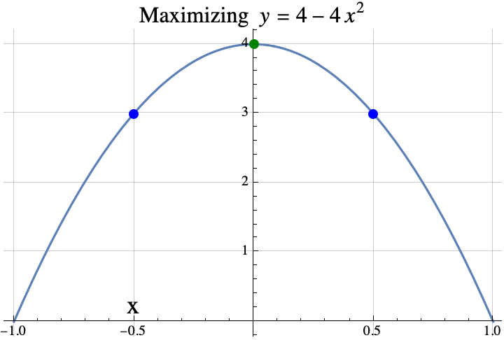
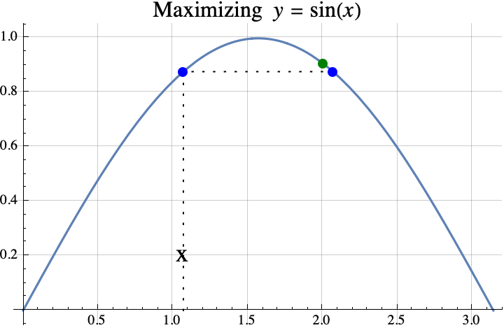
In part 1, we defined the term strictly concave and introduced the theorem that if $f$ is strictly concave and $f(x)=f(x+1)$, then the integer(s) that maximize $f$ are exactly the set $\{\mathrm{floor}(x+1), \mathrm{ceil}(x)\}$ which is usually a set containing only one number $\mathrm{round}(x+1/2)$. In part 2, we showed how the theorem in part 1 can be used to prove that the maximum value that can be obtained when putting an integer into $f(x)=a x^2 + b x + c$ is $f(i)$ where $i=\mathrm{round}(-b/(2a))$ (assuming $a<0$).
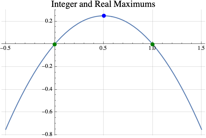
The next theorem says that the real number $x$ that maximizes $f$ is always near the integer $i$ that maximizes $f$.
THEOREM #3
If
- $f$ is a real valued strictly concave function,
- there is a real number $x$ such that $f(x)$ is the maximum value that $f$ attains with real inputs, and
- there is an integer $i$ such that $f(i)$ is the maximum value that $f$ attains with integer inputs,
then $|x-i|<1$.
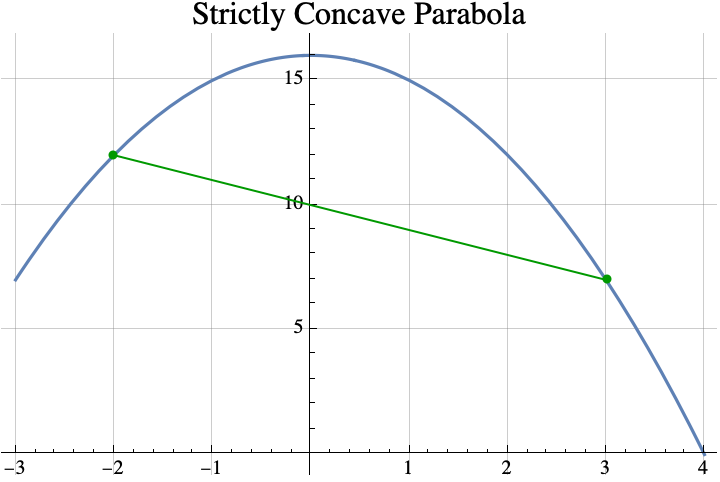
The idea of the proof is fairly simple. Suppose that $i>x+1$. Then $i-1>x$. So $i-1$ is between $i$ and $x$. Concavity implies that that the point $(i-1, f(i-1))$ lies above the line connecting $(x, f(x))$ and $(i,f(i))$, but $f(x)\geq f(i)$.
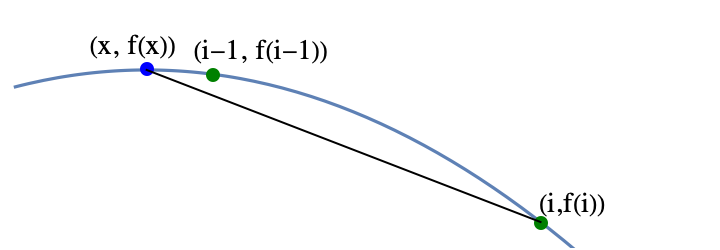
The fact that the point $(i-1, f(i-1))$ is above the line implies that $f(i-1)> f(i)$, but that contradicts the definition of $i$, so using proof by contradiction, $i\leq x+1$. The other cases are either similar or easy.
EXAMPLE
Find the maximum value of $f(x) = x (x-14) (x-20)$ among all integers between 0 and 14.
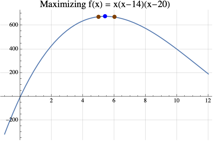
Finding the maximum among reals is easy if you know differential calculus and the quadratic formula. According to differential calculus, the maximum can only occur if the “derivative” of $f(x)$ is zero. $$f(x) = x (x-14) (x-20) =x^3-34 x^2 + 280x.$$ The derivative of a polynomial can be found by multiplying the coefficient by the exponent and decreasing the exponent by 1. The result is $$f'(x) = 3 x^2 -68 x + 280.$$ If we put that in the quadratic formula, we get $$x=\frac{68\pm\sqrt{68^2 – 4 \cdot 3 \cdot 280}}{2 \cdot 3} = \frac{68\pm\sqrt{1264}}{6}\approx 5.41\ \mathrm{or\ } 17.26.$$ It turns out that 17.26 is a local minimum, so the local maximum occurs when $x\approx 5.41$. According to the theorem, any integer $i$ that maximizes $f(i)$ must be within 1 of 5.41, so that integer can only be 5 or 6. Now $f(5)= 675$ and $f(6) = 672$, so 5 is the integer that maximizes $f$. Incidentally, $f(5.41) = 678.025021$ and the true maximum of $f(x)$ is $$f\left(\frac{68-\sqrt{1264}}{6}\right) = \frac{16}{27} \left(442+79 \sqrt{79}\right)\approx 678.025101610626.$$
We could actually use the theorem from part 1 to find the integer $i$ that maximizes $f(i)$. Solving $f(x)=f(x+1)$ using the quadratic formula gives $$x=\frac{1}{6} \left(65\pm\sqrt{1261}\right).$$ If you replace the $\pm$ with the plus sign, you get the local minimum. If you replace it with the minus sign, you get $$\frac{1}{6} \left(65-\sqrt{1261}\right)\approx 4.91.$$ According to the theorem from part 1, the integer that maximizes $f(x)$ must be round(4.91+1/2)=round(5.41)=5. Often it is easier to find the maximum of $f$ rather than trying to solve $f(x)=f(x+1)$, so that is why the theorem above is useful.
If you want to see a more formal mathematical writeup, click here. That PDF shows how you can generalize the three given theorems to a larger class of functions that are not necessarily strictly concave. Also, in the last section of the paper, we sharpen the bound on the difference between the real maximum and the integer maximum. Above, we showed that this difference was less than 1. If $f$ is continuously twice differentiable, then sharper bounds can be computed.
This concludes the three part series.