Articles by hundalhh

Mathematician and Father. Into games, astronomy, psychology and philosophy.

DEFINITION OF THE LAMBERT W FUNCTION

The Lambert W function is a rather unique and useful function that satisfies a special property.

For every non-negative real number $z$, there exists a unique non-negative real number $x$ such that $$x\exp(x) = z.$$

If this condition is satisfied, we say that $x$ is the Lambert W of $z$, and we denote it by $$W_0(z) = x.$$

This function, $W_0$, is the “principal branch” of the Lambert W function. It accepts non-negative real numbers as inputs and provides non-negative real numbers as outputs. We express this in mathematical notation as $W_0:[0,\infty) \rightarrow [0, \infty)$. Alternatively, $W_0$ can be defined as the inverse of the function $$g(x)=x\exp(x).$$

LAMBERT GROWTH RATE

We can use the Lambert W function to solve the delayed growth differential equation $$y'(t) = \beta y(t-T)$$ where $\beta$ and $T$ are positive real numbers.

It is not difficult to show that $$y(t) = \exp(\alpha T)$$ solves the delayed growth differential equation if and only if $$\alpha = W_0(\beta T)/T.$$

We define the Lambert Growth Rate for $\beta$ and $T$ to be $$\mathrm{Lambda\ Growth\ Rate}=\alpha = W_0(\beta T)/T.$$ (Equivalently, $\alpha$ is the unique real number such that the derivative of $y(t) =\exp(\alpha t)$ is $y(t-T)$.)

CALCULATION OR  ESTIMATION

Often, we don’t have the Lambert W function readily available on our calculators or programming environments. So, how do we calculate or approximate it? Let’s look at some methods to compute or estimate this function.  Let’s assume $\beta = 0.2$ and $T=30$ for the methods below.

The various methods for calculating or approximating the Lambert Growth Rate are as follows:

  1. Wolfram Alpha: This is a computational knowledge engine that can be used to solve the equation above directly. You could type "solve a*exp(a*30) = 0.2" into the input box of Wolfram Alpha. The answer given by it would be approximately 0.0477468. Alternatively, to calculate $W_0( \beta T )/T$, you could type "W_0(0.2*30)/30".
  2. Python and Scipy: Python is a popular programming language and scipy is a library for scientific computation in Python. You can use scipy’s implementation from scipy.special import lambertw.
  3. Excel: You can access the Lambert W function with the MoreFunc add-in for Excel.
  4. JavaScript: In Javascript, you can use the math library’s implementation of the Lambert W function. The code would be math.lambertW(x).
  5. Approximations: If you can accept an error of 1 or 2 percent, there are a few approximations available. For instance, if $1.6 \leq x \leq 22$, the Lambert W function can be approximated by the function $$w_1(x) = (.5391 x – .4479)^{(1/2.9)}.$$ We can use this approximation to estimate the growth rate
    $$W_0( 30*0.2)/30= W_0(6)/30\approx (.5391\times 6 – .4479)^{(1/2.9)}/30\approx 0.047463321.$$ Also, if $0\leq x \leq 2$, another approximation function is $$w_2(x) = \frac{x}{(1+x)(1-0.109 x)}.$$
  6. Bisection MethodWe want to find the value of $\alpha$ where $$\alpha \exp(\alpha T) = \beta.$$ That value of $\alpha$ is the “root” of the function $$f(\alpha)=\alpha \exp(\alpha T) – \beta.$$ A root of a function $f(\alpha)$ is any $\alpha$ where $f(\alpha)=0$.  The bisection method continuously splits an interval in half to narrow down the root of a function. It assumes the function changes sign around the root, and iteratively refines the search interval.  In our case, $f(0)= -\beta<0$ and $$f(\beta) = \beta\exp(T\beta) -\beta>0,$$ so we know that $\alpha=0$ is too low and $\alpha=\beta$ is too high.  The bisection method would now test the midpoint of the interval $[0,\beta]$ which is $\beta/2.$  If $f(\beta/2)>0$ the bisection method begins again on the interval $[0,\beta/2]$ and if $f(\beta/2)<0$ the bisection method would continue with the interval $[\beta/2, \beta]$. Every iteration cuts the size of the interval in half.
  7. Newton-Raphson Method: The Newton-Raphson method is a popular root-finding algorithm that uses tangents to the function to find the roots. It can be used to improve the accuracy of the approximations above. The formula for estimating the solution of $f(x)=0$ is $$n(x) = x – f(x)/f'(x).$$For our problem $$n(x) = x-\frac{x e^{T x}-\beta}{(T x +1)e^{T x}}.$$

Simulation


In the game Master of Orion, the economic growth rate in the early part of the game can be estimated by $\alpha=W_0(T\frac{I}{C})$ where $I$ represents the income of a “mature” planet, $C$ is the cost of constructing a colony ship, $T$ is the number of years between the construction year of a colony ship and the year that the colonized planet is “mature”. I ran a simulation using typical but random values where $10\leq I\leq200$, $200\leq C\leq575$, and $10\leq T\leq90$. Every time I generated random $I$, $C$, and $T$ values, I would use either $w_1$ or $w_2$ to estimate the Lambert growth rate $W_0(TI/C)/T$. Let $x= TI/C$. If $x<1.8$, I used $w_2$ and I used $w_1$ otherwise. The average error using $w_1$ and $w_2$ was 0.0016. If I then applied $n$ to the approximation, then the average error was 0.00017, about 10 times more accurate. When I applied $n$ twice the average error dropped to 0.000005 and the worst case error was 0.0001. If you want 16 digits of accuracy, you need to apply the function $n$ five times.

Applying the Newton Raphson to estimate the Lambert growth rate for $T=30$ and $I/C = \beta = 0.2$ and, gives
$$
\begin{aligned}
W_0(I T/C)/C = W_0(6)/30 \approx w_1(6)/30 &\approx 0.047463321\\
W_0(6)/30 \approx n(w_1(6)/30) &\approx 0.047748535122\\
W_0(6)/30 \approx n(n(w_1(6)/30)) &\approx 0.047746825925 \\
W_0(6)/30&\approx 0.047746825863
\end{aligned}
$$

Summary

In this post we presented several methods for approximating the Lambert Growth Rate $$W_0(\beta T)/T.$$ If you don’t have Wolfram Alpha or access to a programming environment that includes the Lambert W function, then one of the best methods for finding the solution is the Bisection Method.  If $x=\beta T<100$, then using $w_1$ or $w_2$ approximates the solution to within 2%.  One iteration of Newton-Raphson typically reduces the error by a factor of 10.  More iterations of Newton-Raphson significantly improve the approximation.


In Part 1, we defined the Second Banker’s problem and gave a formula for the optimal time to make a purchase.  All of the proofs are given in this PDF.


Interest Income immediately before the optimal purchase time for the Second Panker’s problem

As with the first banker’s problem, the income from interest just before the optimal purchase time is
$$
\mathrm{interest\ income\ during\ purchase} = \frac{c \;r_1 r_2 }{r_2-r_1}.
$$

Notice that this income does not depend on the initial amount in the bank account $B_0$.

For example, if

  • you initially have \$1000 in the account,
  • the cost of increasing the interest rate is \$1,100,
  • $r_1=0.05=5\%$, and
  • $r_2=0.08=8\%$,

then $$\begin{aligned}\mathrm{interest\ income\ during\ purchase} &= \frac{c \;r_1 r_2 }{r_2-r_1}\\&= \frac{ \$1100\cdot 0.05 \cdot 0.08}{0.08-0.05}\\&= \frac{ \$55 \cdot 0.08}{0.03} \approx \$146.67\mathrm{\ per\ year.}\end{aligned}$$

REMARK

Note that the interest income can also be expressed by
\begin{equation}
\label{eqone}
\mathrm{interest\ income\ during\ purchase} = c/t_{\mathrm{pay}}
\end{equation}
where
\begin{equation}
\label{eqtwo}
t_\mathrm{pay} = \frac1{r_1} – \frac1{r_2}= \frac{c}{B_0 r_1 \exp(r_1 t_\mathrm{buy})}
\end{equation}
is the amount of time it takes to pay $c$ dollars from interest starting at the optimal time $t_\mathrm{buy}$.

For the previous example, we get
$$
t_\mathrm{pay} = \frac1{r_1} – \frac1{r_2} = \frac1{0.05} – \frac1{0.08} = 20 – 12.5 = 7.5\mathrm{\ years,\ and}
$$
$$
\mathrm{interest\ income\ during\ purchase} = c/t_{\mathrm{pay}}= 1100/7.5 \approx \$146.67/\mathrm{year}.
$$


Recovery Time

If you do purchase the interest rate hike at the optimal time, how many years will you need to wait until the optimal strategy surpasses the never buy strategy. The recovery time for the second banker’s problem is almost, but not quite the same as the first banker’s problem. For the second banker’s problem,
$$
t_{\mathrm{surpass}} = t_{buy} + 1/r_1.
$$
For the example,
$$
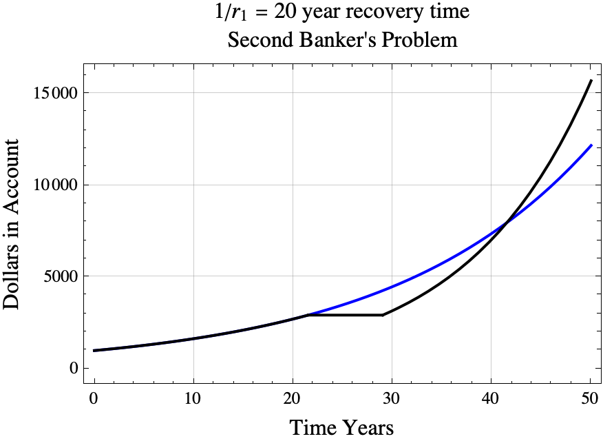
t_{\mathrm{surpass}} \approx 21.5228+ \frac{1}{0.05} = 41.5228.
$$

SecRecover

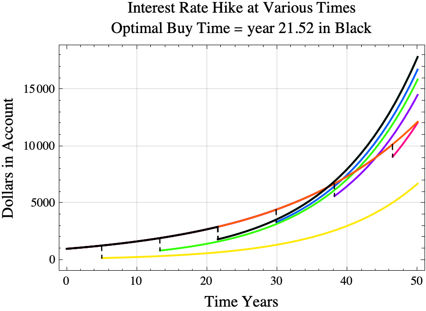
The black line shows the results of buying the interest rate increase at the optimal time. The blue line shows what happens if you never buy the interest rate hike and just continue to get 5% interest.
If you buy the interest rate hike at the optimal time, then you will maximize the account balance at all times $t>1/r_1$ years later. (Mathematically, for every $t> t_{\mathrm{buy}} + 1/r_1$, the strategy of purchasing the interest rate upgrade at time $t_{\mathrm{buy}}$ results in an account balance at time $t$ that exceeds the account balance at time $t$ using any other strategy.)

Consider the following game. You have a bank account that is compounded continuously with an interest rate of $r_1$. Your banker offers you the following deal. At any time in the future, you can pay $c$ dollars using only the interest from the account to increase your interest rate to $r_2$. If your balance is $b$ at the time of the upgrade, then your balance will remain at $b$ for $c/(r_1 b)$ years which is the time required to pay $c$ dollars from interest alone.  Other than paying for the interest upgrade, you can never add or subtract any money until retirement which is very far in the future. When should you accept the banker’s offer? Let’s call this game “the second banker’s problem”. (We assume that $c, r_1,$ and $r_2$ are positive real numbers and $1>r_2> r_1>0$.)

(This game is similar to purchasing a growth technology in the game Master of Orion (Original 1993 version).  For example, if you buy the “Improved Industrial Tech 9″ technology early in the game, the cost of factories is reduced for the remainder of the game. Reducing the cost of factories increases your economy’s growth rate.)

(All proofs for the second banker’s problem can be found in this PDF.)

 
For the first banker’s problem, the balance in the account is immediately reduced by $c$ dollars and the interest rate is immediately increased to $r_2$. See this blog post or this PDF for an analysis of the first banker’s problem. The third banker’s problem allows the saver to buy two separate interest rate increases.

 
For the second banker’s problem, you might be tempted to say that you should buy the interest rate increase as early as possible, but that might be bad if $c/(r_1 b)$ is a large number of years.  On the other hand, there is no reason to buy the interest rate upgrade if the time to retirement is less than $c/(r_1 b)$ years.

Optimal Purchase Time

Perhaps surprisingly, the optimal time to purchase the interest rate hike is the same for the first and the second banker’s problems. For either problem, you should take the deal at time
$$t_{\mathrm{buy}}=\frac{1}{r_1}\ln\left(\frac{c \; r_2 }{B_0(r_2-r_1)}\right)$$
where $B_0$ is the amount of money in the account at time zero, and $\ln(x)$ is the natural log. $$\ln(x) = \frac{\log_{10}(x)}{\log_{10}(e)}.$$ I was a bit surprised to find that the optimal purchase time $t_{\mathrm{buy}}$ for the second banker’s problem is the same as the optimal purchase time for the first banker’s problem.

The amount of money in the account at the optimal purchase time is $$b_{\mathrm{opt}} = \frac{c \; r_2 }{r_2-r_1}.$$

Example

For example, if

  • you initially have \$1000 in the account,
  • the cost of increasing the interest rate is \$1,100,
  • $r_1=0.05=5\%$, and
  • $r_2=0.08=8\%$,

then the the correct time to buy the interest rate increase is
$$
\begin{aligned}
t_{\mathrm{buy}}&=\frac{1}{r_1}\ln\left(\frac{c \; r_2 }{B_0(r_2-r_1)}\right)\\
&=\frac{1}{0.05}\ln\left(\frac{1100\cdot 0.08 }{1000(0.08-0.05)}\right)\\
&=\frac{1}{0.05}\ln\left(\frac{88 }{1000(0.03)}\right)\\
&=20\ln\left(\frac{88 }{30}\right)\\
&\approx21.5228\ \mathrm{years.}
\end{aligned}
$$

SecondBanker

SecondBLegend


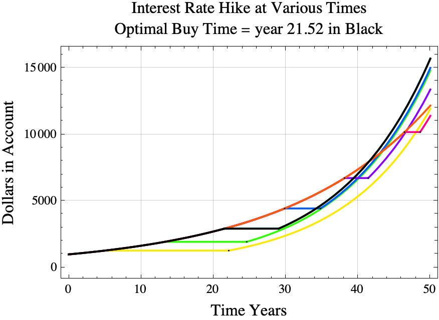
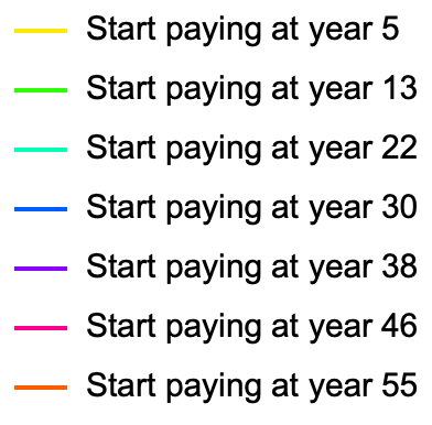
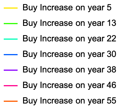
In the diagram above, the black line shows the results of paying \$1,100 from interest starting at year 21.5228, the optimal time to start paying for the interest rate upgrade. The orange line shows what happens if the player does not invest before year 50. The yellow line shows the result if she or he starts paying for the investment on year 5.

In part 1, we described the “first banker’s problem” where you can pay a banker to increase your interest rate from $r_1$ to $r_2$ by removing $c$ dollars from your account.  The optimal time to purchase the rate increase is when you have

\begin{equation}
\mathrm{balanceBefore} =\frac{c \; r_2 }{r_2-r_1}
\end{equation}

dollars in your account.  (All of the formulas and theorems about the first banker’s problem as well as Python simulation code for the first banker’s problem and proofs can be found in this PDF.)


Interest Income immediately before the optimal purchase time

When compounding continuously, the amount of interest that you are earning at any time is the balance at that time times $r_1$.  The amount of interest income just before the optimal purchase time is

$$\mathrm{interst\ income\ immediately\ before\ purchase} = r_1\cdot \mathrm{balanceBefore} = \;\frac{r_1 r_2  c}{r_2-r_1}.$$

example

If

  • you initially have \$1000 in the account,
  • the cost of increasing the interest rate is \$1,100,
  • $r_1=0.05=5\%$, and
  • $r_2=0.08=8\%$,

then
$$
\begin{aligned}
\mathrm{income\ immediately\ before\ purchase} &= \frac{c \;r_1 r_2 }{r_2-r_1}\\
&= \frac{ \$1100\cdot 0.05 \cdot 0.08}{0.08-0.05}\\
&= \frac{ \$55 \cdot 0.08}{0.03} \approx \$146.67\mathrm{\ per\ year.}
\end{aligned}
$$

Recovery Time

If you do purchase the interest rate hike at the optimal time, how many years will you need to wait until the optimal strategy surpasses the never buy strategy? The answer is you will have to wait approximately $1/m$ years after the purchase where $m$ is the average of $r_1$ and $r_2$.  The exact time when the optimal strategy surpasses the never buy strategy is

$$
t_{\mathrm{surpass}} = t_{buy} + \frac{ \ln(r_2) – \ln(r_1)}{r_2-r_1}.
$$where $$t_{\mathrm{buy}}=\frac{1}{r_1}\ln\left(\frac{c \; r_2 }{B_0(r_2-r_1)}\right)$$

and $B_0$ is the amount in the account at time 0.  (Bounds for the expression $(\ln(r_2) – \ln(r_1) )/ (r_2 – r_1)$ can be found here.)

For the previous example,

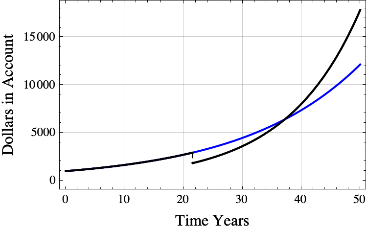
$$t_{\mathrm{surpass}} \approx 21.5228+ \frac{ \ln(0.08) – \ln(0.05)}{0.08-0.05} \approx 37.1868.$$

BSurp

The black line shows the results of buying the interest rate at the optimal time. The blue line shows what happens if you never buy the interest rate hike and just continue to get 5% interest.

The number of years needed to catch up is between $1/r_2$ years and $1/r_1$ years. GPT wrote a nice proof of this fact.

If you buy the interest rate hike at the optimal time, then you will maximize the account balance at all times $t>1/r_1$ years later. (Mathematically, for every $t> t_{\mathrm{buy}} + 1/r_1$, the strategy of purchasing the interest rate upgrade at time $t_{\mathrm{buy}}$ results in an account balance at time $t$ that exceeds the account balance at time $t$ using any other strategy.

In the game Master of Orion and some related games, it is possible to purchase technologies that increase the rate of growth of your empire.  I wanted to simplify this idea enough to get clean mathematical solutions.  I call the resulting three simplified games the first, second, and third banker’s problems.

  1. In the first banker’s problem, the saver is offered a deal where they can buy an interest rate upgrade for a fixed amount of money paid from the account balance at any time specified by the saver.
  2. The second banker’s problem is the same as the first, except that the payment for the interest upgrade comes solely from account interest.
  3. For the third banker’s problem the saver can, at any time, upgrade from interest rate $r_1$ to interest rate $r_2$ for $c_1$ dollars and upgrade from $r_2$ to $r_3$ for $c_2$ dollars, or upgrade directly from interest rate $r_1$ to interest rate $r_3$ for $c_2$ dollars where $r_1<r_2<r_3$ and $c_1<c_2$.

This post will state the formula for computing the optimal time to buy the interest rate upgrade for the first banker’s problem, compute the optimal time to buy for one example, and show the results of buying at non-optimal times.

All of the formulas and theorems about the first banker’s problem as well as Python simulation code for the first banker’s problem and proofs can be found in this PDF.


the first banker’s problem

Consider the following game. You have a bank account that is compounded continuously with an interest rate of $r_1$. Your banker offers you the following deal. At any time in the future, if your account balance is greater than $c$ dollars, you can pay $c$ dollars from the account to increase your interest rate to $r_2$. You can only use the funds in the account to pay for this interest rate increase and you can never add or subtract any money until retirement which is very far in the future. When should you accept the banker’s offer?  (We assume that $c, r_1,$ and $r_2$ are positive real numbers and $1>r_2> r_1>0$.)

At first you might be tempted to say that you should buy the interest rate increase as early as possible, but it turns out that that is a bad idea. If you have exactly $c$ dollars in the account and you buy the rate increase, then you will have zero dollars in the account and you are stuck with zero dollars in the account until you retire. Similarly, if you have $c+\$0.01$ in the account and you buy the interest rate increase, then you will only have one cent in the account after the purchase, and it will take a long time to grow that one cent into a large amount of money.

On the other hand, it is probably wrong to wait until the last microsecond before you retire to buy an interest rate increase because the increased amount of interest that you receive is unlikely to be larger than the cost $c$.

The answer to the first banker’s problem is that you should take the deal at time

\begin{equation}
t_{\mathrm{buy}}=\frac{1}{r_1}\ln\left(\frac{c \; r_2 }{B_0(r_2-r_1)}\right)
\end{equation}
where $B_0$ is the amount of money in the account at time zero, and $\ln(x)$ is the natural log. $$\ln(x) = \frac{\log_{10}(x)}{\log_{10}(e)}.$$

At that time the balance before the purchase will be

\begin{equation}
\mathrm{balanceBefore} =\frac{c \; r_2 }{r_2-r_1},
\end{equation}

and the balance immediately after purchasing the interest upgrade will be

\begin{equation}
\mathrm{balanceAfter} =\frac{c \; r_1 }{r_2-r_1}.
\end{equation}


Example

For example, if

  • you initially have \$1000 in the account,
  • the cost of increasing the interest rate is \$1,100,
  • $r_1=0.05=5\%$, and
  • $r_2=0.08=8\%$,

then the the correct time to buy the interest rate increase is

$$
\begin{aligned}
t_{\mathrm{buy}}&=\frac{1}{r_1}\ln\left(\frac{c \; r_2 }{B_0(r_2-r_1)}\right)\\
&=\frac{1}{0.05}\ln\left(\frac{1100\cdot 0.08 }{1000(0.08-0.05)}\right)\\
&=\frac{1}{0.05}\ln\left(\frac{88 }{1000(0.03)}\right)\\
&=20\ln\left(\frac{88 }{30}\right)\\
&\approx21.5228\ \mathrm{years}
\end{aligned}
$$and the account balance before making the payment at the optimal time would be

$$\begin{aligned}\mathrm{balanceBefore} &=\frac{c \; r_2 }{r_2-r_1}\\&=\frac{1100 \cdot 0.08 }{0.08-0.05}\\&=\frac{88 }{0.03}\\&\approx \$2933.33.\end{aligned}$$

The diagram below shows what happens if you buy the interest upgrade at various times.  The purchases are represented as a black vertical dashed lines. The solid black line shows the results of paying \$1,100 at year 21.5228, the optimal time to invest. The red line shows what happens if the player does not invest before year 50. The yellow line shows the result if she or he invests on year 5.


Banker BLegend


The following function has come up twice in my research

$$f(a,b)=\frac{\ln(b)-\ln(a)}{b-a}$$ where $0<a<b.$

Now, I had known that if $a$ and $b$ are close, then $$f(a,b)\approx\frac{1}{\mathrm{mean}(a,b)}$$ and $$\frac{1}{b}<f(a,b)<\frac1{a}.$$ But last week, with a little help from GPT, I got some better approximations and bounds on $f(a,b)$.

Let $m=(a+b)/2$ and $\Delta = (b-a)/2$.

Below GPT and I derive the following

  • $$1/b < f(a,b) < 1/a,$$
  • $$1/m <  f(a,b) < 1/m + \frac{\Delta^2}{3m}\left(\frac{1}{m^2-\Delta^2 }\right),$$
  • $$ -\frac{2\Delta^4}{15a^5}< f(a,b)\; – \frac{1}{6}\left(\frac{1}{a}+\frac{4}{m}+\frac{1}{b}\right) < -\frac{2\Delta^4}{15b^5},\mathrm{\ and}$$
  • $$\begin{aligned} f(a,b) &= \frac{ \tanh^{-1}(\Delta/m)}{\Delta} = \frac1{m} \frac{ \tanh^{-1}(\Delta/m)}{\Delta/m}\\&= \frac{1}{\Delta} \left(\frac{\Delta}{m} + \frac{\Delta^3}{3m^3}+ \frac{\Delta^5}{5m^5} + \cdots\right)\\  &= \frac{1}{m} \left(1 + \frac{\Delta^2}{3m^2}+ \frac{\Delta^4}{5m^4} + \cdots\right) \end{aligned}$$

where  $$ \tanh^{-1}(y) = x$$ if and only if $$\tanh(x) := \frac{ e^x-e^{-x}}{e^x + e^{-x}} =y$$ for any $x\in\mathbb{R}$ and $y\in(-1,1)$.

(Alternatively, $$\tanh^{-1}(x) = \frac{1}{2} \ln (x+1)-\frac{1}{2} \ln (1-x)$$ where $\ln(x)$ is the natural log and $|x|<1$.)

The derivation

At first I tried to use Taylor Series to bound $f(a,b)$, but it was a bit convoluted so I asked GPT. GPT created a much nicer, simpler proof. (See this PDF). GPT’s key observation was that $$f(a,b)= \frac{\ln(b)-\ln(a)}{b-a} = \frac{1}{b-a}\int_a^b \frac{dx}{x}$$ is the mean value of $1/x$ over the interval $[a,b]$. (In truth, I felt a bit dumb for not having noticed this. Lol.)

GPT’s observation inspires a bit more analysis.

Let $$z= \frac{x}{m} -1,\mathrm{\ so\ \ } m(z+1)=x.$$ If $x=a$, then
$$z= \frac{a}{m} -1= \frac{m-\Delta}{m} – 1= -\frac{\Delta}{m}.$$
Similarly, if $x=b$,
$$z= \frac{b}{m} -1= \frac{m+\Delta}{m} – 1= \frac{\Delta}{m}.$$
Applying these substitutions to the integral yields
$$\begin{aligned}
\int_{x=a}^{x=b} \frac{dx}{x} &=\int_{z=-\Delta/m}^{z=\Delta/m}\frac{m\;dz}{m(z+1)} \\
&=\int_{z=-\Delta/m}^{z=\Delta/m}\frac{dz}{z+1} \\
&=\int_{z=-\Delta/m}^{z=\Delta/m} (1-z+z^2-z^3+\cdots)dz\\
&=\int_{z=-\Delta/m}^{z=\Delta/m} (1+z^2+z^4+\cdots)dz\\
&=\int_{z=-\Delta/m}^{z=\Delta/m} \frac{dz}{1-z^2}\\
&=\left.\tanh^{-1}(z)\right|_{z=-\Delta/m}^{z=\Delta/m} \\
&= \tanh^{-1}(\Delta/m) – \tanh^{-1}(-\Delta/m)\\
&= 2 \tanh^{-1}(\Delta/m).
\end{aligned}$$
(Above we twice applied the wonderful thumb rule $$\frac{1}{1-x} = 1+ x + x^2 +x^3+\dots$$ if $|x|<1$. See idea #87 from the top 100 math ideas.)

So,
$$\frac{\ln(b) – \ln(a)}{b-a} =\frac{ 2 \tanh^{-1}(\Delta/m)}{b-a}=\frac{ \tanh^{-1}(\Delta/m)}{\Delta}.$$

Furthermore,
$$
\tanh^{-1}(x) = x + x^3/3 + x^5/5 + \cdots,
$$
so
$$\begin{aligned}
f(a,b) = \frac{\ln(b) – \ln(a)}{b-a} &= \frac{1}{\Delta} \left(\frac{\Delta}{m} + \frac{\Delta^3}{3m^3}+ \frac{\Delta^5}{5m^5} + \cdots\right) \\
&=\frac{1}{m} + \frac{\Delta^2}{3m^3}+ \frac{\Delta^4}{5m^5} + \frac{\Delta^6}{7m^7} + \cdots
\end{aligned}$$
This series gives us some nice approximations of $f(a,b)$ when $\Delta/m<1/2$. We can also bound the error of the approximation $$f(a,b)\approx 1/m$$ as follows $$\begin{aligned}
\frac{1}{m} <\frac{\ln(b) – \ln(a)}{b-a}&=\frac{1}{m} + \frac{\Delta^2}{3m^3}+ \frac{\Delta^4}{5m^5} + \frac{\Delta^6}{7m^7} + \cdots \\
&<\frac{1}{m} + \frac{\Delta^2}{3m^3}+ \frac{\Delta^4}{3m^5} + \frac{\Delta^6}{3m^7} + \cdots \\
&=\frac{1}{m} + \frac{\Delta^2}{3m^3}(1 + \frac{\Delta^2}{m^2} + \frac{\Delta^4}{m^4} + \cdots )\\
&=\frac{1}{m} + \frac{\Delta^2}{3m^3}\left(\frac{1}{1-\frac{\Delta^2}{m^2} }\right)\\
&=\frac{1}{m} + \frac{\Delta^2}{3m}\left(\frac{1}{m^2-\Delta^2 }\right).\\
\end{aligned} $$

Example.

Let $a= 6/100$ and $b=7/100$. Then $m=13/200$, $\Delta = 1/200$,

  • $$\frac{\ln(b)-\ln(a)}{b-a}= \tanh^{-1}(\Delta/m)/\Delta \approx 15.415067982725830429,$$
  • $$1/m \approx 15.3846,$$
  • $$1/m + \Delta^2/(3 m^3)\approx 15.41496,\ \mathrm{and}$$
  • $$1/m + \Delta^2/(3 m^3) + \Delta^4/(5 m^5)\approx 15.4150675.$$
  • $$1/m+ \frac{\Delta^2}{3m}\left(\frac{1}{m^2-\Delta^2 }\right)\approx 15.41514$$


Applying Simpson’s Rule

We can also use Simpson’s rule to approximate $\ln(b)-\ln(a)$.  The error formula for Simpson’s rule is

$$\begin{align}\int_{a}^{b}g(x)\,dx&=\frac{\Delta}{3}[g(a)+4g(m)+g(b)]-\frac{\Delta^5}{90}g^{(4)}(\xi)\end{align}$$

for some $\xi$ in the interval $(a,b)$. Setting $g(x)=1/x$, $$I=\ln(b)-\ln(a),\quad\mathrm{ and }\quad h(a,b)= \frac{\Delta}{3}\left(\frac{1}{a}+\frac{4}{m}+\frac{1}{b}\right)$$ with $m=(a+b)/2$ and $\Delta=(b-a)/2$ gives

$$\begin{align} \ln(b) – \ln(a) &=\frac{\Delta}{3}\left(\frac{1}{a}+\frac{4}{m}+\frac{1}{b}\right)-\frac{\Delta^5}{90}\frac{24}{\xi^5} \\ I&=h(a,b)-\frac{4\Delta^5}{15\xi^5}\\I-h(a,b) &= -\frac{4\Delta^5}{15\xi^5}\\-\frac{4\Delta^5}{15a^5}&< I-h(a,b) < -\frac{4\Delta^5}{15b^5}.\end{align}$$

Now we divide by $2\Delta = b-a$ to conclude that
$$\begin{aligned}\frac{\ln(b) – \ln(a)}{b-a}&= \frac{1}{6}\left(\frac{1}{a}+\frac{8}{a+b}+\frac{1}{b}\right) + error \\&= \frac{1}{6}\left(\frac{1}{a}+\frac{4}{m}+\frac{1}{b}\right) + error \\&\approx \frac{1}{6}\left(\frac{1}{a}+\frac{4}{m}+\frac{1}{b}\right) -\frac{2\Delta^4}{15m^5}\end{aligned}$$
where
$$ -\frac{2\Delta^4}{15a^5}< error < -\frac{2\Delta^4}{15b^5}.$$


(Thanks to GPT and StackEdit(https://stackedit.io/).)


The game Master of Orion, first released in 1995 by Microprose, entails settling the galaxy planet by planet.  To settle a planet, the player must construct a colony ship on one of her/his planets, send that ship to a new, unoccupied habitable planet, land the ship, and then send colonists from some of their planets to the new planet.  Early in the game,

  • it costs about 550 MC to build the colony ship,
  • it takes around 5 turns for the colony ship to reach a new planet,
  • it takes and additional 5 turns for additional colonists to arrive on the planet on separate (free) transport ships,
  • it takes around 20 turns for the planet to build new factories before it can build new colony ships, and
  • the new planet might generate 110 MC per turn of income to build more ships,

so 30 turns after investing 550 MC, the player’s income increases by about 110 MC per turn.

If we try to create a differential equation to model the early stage of the game, we get something like

$$y'(t) = \frac{110}{550} y(t-30) = \frac{1}{5}y(t-30) $$

where $y(t)$ is the income available for building ships on turn $t$. This differential equation has a solution of the form $$y(t) = c \exp(\alpha t).$$ We can compute the derivative and substitute into the differential equation to find $\alpha$.

$$y'(t) = c\alpha \exp(\alpha t).$$

So,
$$\begin{aligned} c\alpha \exp(\alpha t) &= y'(t) =\frac{1}{5} y(t-30)\\c\alpha \exp(\alpha t) &=\frac{1}{5}c \exp(\alpha(t-30)) \\\alpha &=\frac{1}{5} \exp(-30 \alpha) \\\alpha \exp(30 \alpha) &=\frac{1}{5}\\30 \alpha \exp(30 \alpha) &= 6 \end{aligned}$$
According to the definition of the Lambert W function $W_0(x)$ for $x>0$,
$$ W_0(z) = x$$
if and only if
$$ x\exp(x) = z.$$
Setting $x=30\alpha$ above gives
$$\begin{aligned}W_0(6) &= 30\alpha\\ W_0(6)/30 &=\alpha\\ \alpha &= W_0(6)/30\approx 0.0477468.\end{aligned}$$
So the the economy at the start of the Master of Orion gain should grow by about 5% per year.

More generally, if

– the time between the investment in the colony ship and the maturing of the colonized planet is $T$,
– the cost of the ship is $C$,
– and the mature planets produces $i$ income per turn,
then the income on turn $t$ can be approximated by $$y(t) = y(0) \exp(\alpha t)$$ where
$$\alpha = \frac{W_0\left(\frac{i T}{C}\right)}{T}.$$

(Thanks to stackedit.io for helping me format the TeX.)

Last month I wrote a post about the fact that you should not make an investment in a game that does not pay for itself.  If an investment costs $I$ and gives you a return of $i$ per turn, then it will pay for itself in $I/i$ turns.  The return on investment (ROI) is $$r= i/I.$$ In some games we have several choices about how to invest, and generally speaking it is best to choose the investments with the best ROI.

If you can invest on any turn, the ROI investment rule of thumb is,

“Don’t invest if there are less than $$I/i=1/r$$ turns in left in the game excluding the current turn.”


the tank game

The tank game is one of the simplest investment games.  It illustrates a few common ideas in investment games:

  • Exponential Sharpening of the Axe
  • The optimal investment choice often depends only on the ROI for the turn and the number of turns left in the game.
  • Solving an investment game often involves finding the largest rectangle under the investment curve.
  • The investment-exploitation phase transition, dominating strategies, comparing two very similar strategies, null moves, and strategy swaps
  • Actually proving that a strategy is correct is a bit tricky.
  • Discrete vs. Continuous.

I will address some of these ideas in this post and the rest of the ideas in a follow up post.


Suppose that you start the game with an income of \$100 million per turn.  Each turn you have the two choices:

  • (investment option) investing all your income into factories and increasing your income by 10%, or
  • (don’t invest option) building tanks that cost one million dollars each.

Assume that it is also possible to build half a tank, or any other fraction of a tank, so if you spend \$500,000 on tanks, you get 0.5 tanks. If you spend \$2,300,000 on tanks, then you get 2.3 tanks. The game lasts for 27 turns and the object of the game is to maximize the number of tanks created.

Intuitively, you want to build up your factories in the first part of the game (Invest/Growth phase), and then transition to making tanks in the later part of the game (Exploitation phase).

Suppose that you build factory equipment for the first 5 turns, and then spend 22 turns building tanks.  After the first turn, you have \$110 million income (\$100 million original income plus \$10 million income due to the investment into factory equipment). After the second turn, your income would be \$121 million (\$110 million at the start of the turn plus \$11 million additional income due to investment). After the third turn you would have \$133,100,00 income, the fourth \$146,410,000 income, and finally, at the end of the 5th turn, your income would be \$161,051,000 per turn. If you then build tanks for 22 turns, then you would have $$22\cdot161.051 = 3543.122\ \ \mathrm{tanks}$$ at the end of the game.


The optimal strategy for the tank game using the rule  of thumb

The easy way to find the optimal strategy is to apply the ROI investment rule of thumb.  We should invest as long as there are more than $I/i=1/r$ turns in the game after the current turn.  In the tank game, you increase your income by 10% if you invest, so $r=0.10$ and $$1/r=10\ \ \mathrm{turns.}$$ On turns 1 through 16 there are more than 10 turns left in the game, so you must invest on those turns.  On turn 17, there are exactly 17 turns left in the game, so it does not matter whether or not you invest on that turn.  On turns 18, 19, … 27, there are less than 10 turns left in the game, so on those turns, you need to build tanks.

If you do invest for 17 turns, then your income would be $$\mathrm{income} = (1.1)^{17}\cdot \ \$100,000,000= \$ 505,447,028.50$$ per turn.  Then you could buy tanks for 10 turns giving you about 5054.47 tanks.

OptTank

Notice that the amount of money spent on tanks is the same as the area of a rectangle with height equal to the income at the end of the investment phase (turn 17) times the number of turns used to buy tanks.  Many investment problems are equivalent to finding the largest rectangle that “fits” under the income curve.


The investment-exploitation phase transition and dominating strategy swaps

If you actually want to prove that this is the optimal strategy, you should probably first prove that there is and investment phase followed by a building/exploitation phase.

We will prove that investment phase must come first by comparing two very similar strategies where we swap a Building action and an Investing action. Comparing two similar strategies and showing the one “dominates” the other is a common tactic for finding optimal strategies.  In game theory, we say that one strategy dominates another if it is always better no matter what the opponent does.  For the single player tank game, we will say that one strategy dominates another if it produces more tanks over the course of the game.

Option 1:  Build-then-Invest. Suppose that on turn $i$ that you build tanks and on turn $i+1$ you invest in factories.  Suppose that on turn $i$ that your income was $I$.  Then you would build $$\mathrm{tanks} = \frac{I}{\$1,000,000}$$ tanks on turn $i$ and your income would increase to on turn $i+1$ to $$I_{\mathrm{new}}=1.1\ I.$$

Option 2:  Invest-then-Build.  On the other hand, if you swap the two strategies on turns $i$ and $i+1$, then on turn $i$ your income would again increase to $$I_{\mathrm{new}}=1.1\ I,$$ but when you build the tanks on turn $i+1$ you end up with  $$\mathrm{tanks} = \frac{I_{\mathrm{new}}}{\$1,000,000}= \frac{1.1\ I}{\$1,000,000}.$$

For either option, you have the same income on turns $i+2, i+3, \ldots, 27$, but for Option 2 (Invest-then-build) you have 10% more tanks than option 1.  We conclude that Option 2 “dominates” option 1, so for the optimal strategy, a tank building turn can never precede an investment turn.  That fact implies that there is an investment phase lasting a few turns followed by an building phase where all you do is build tanks.

If we carefully apply the ideas in the ROI part 1 post, we can determine where the phase transition begins. Suppose that on turn $i$ we have income $I$ and we make our last investment to bring our income up to $1.1\ I$. The increase in income is $0.1\ I$ and that new income will buy $$\mathrm{tanks\ from\ new\ income} = \frac{0.1\  I (T-i)}{\$1,000,000}$$ new tanks where $T=27$ is the total number of turns in the game.  If we build tanks instead of investing on turn $i$ then we would make $$\mathrm{potential\ tanks\ on\ turn\ }i = \frac{I}{\$1,000,000}$$ tanks.  The difference is
$$\begin{aligned} \mathrm{gain\ by\ investing} &=  \frac{0.1\ I (T-i)}{\$1,000,000}\;  – \frac{I}{\$1,000,000}\\ &= \frac{0.1\ (T – i) \;- I}{\$1,000,000}.\end{aligned}$$

The gain is positive if and only if $$\begin{aligned} 0.1\ I (T-i) – I &> 0\\ 0.1\ I (T-i) &> I\\ 0.1\ (T-i) &> 1\\T-i &> 10\\T-10&> i.\end{aligned}$$

Remark: Reversing the inequalities proves that  the gain is negative ( a loss) if and only if    $T-10 < i$.

We conclude that no tanks can be built before turn $T-10=17$.  On turn $i=17$, $$0.1\ I (T-i) -I = 0.1\ I (27-17) -I =  0,$$ so the gain by investing is zero. It does not matter whether the player builds tanks or invests on turn 17.  After turn 17, the gain is negative by the Remark above, so you must build tanks after turn 17.

We have proven that the ROI investment rule of thumb works perfectly for the tank game.

In the previous 5 parts, I described several theorems which are useful for finding the maximum value of a function $f$ over integers.  In parts 1, 2, and 3, $f$ was concave.  In part 4, $f$ was continuous.  And in part 5, there were no restrictions on $f$.  In this post, the focus is on finding the maximum value of an investment game function over integers.

What is the maximum of $$f(x)=\exp(\alpha x) (T-x)$$ over all integers?  This function appears in several investment board games including Terraforming Mars, Master of Orion, and Roll for the Galaxy.

EXAMPLE $f(x)=\exp(\alpha x) (T-x)$

Let’s find the maximum of $f:\mathbb{R}\rightarrow\mathbb R$ where $$f(x)=\exp(\alpha x) (T-x),$$ $\alpha>0$, and $T>0$. The $\exp(\alpha x)$ is always postive, so $$f(x)>0\quad\mathrm{\ if\ and\ only\ if\ } x<T.$$

Let $g(x) = f(x+1) – f(x)$ as in “Maximizing a Function over Integers (Part 5)“. Let $\beta=\exp(\alpha)$. We can use some algebra to better understand the behavior of $g$.

$$\begin{aligned}g(x) &= f(x+1) – f(x)\\&= \exp(\alpha (x+1)) (T-(x+1)) – \exp(\alpha x) (T-x)\\&= \beta\beta^x (T-x -1) – \beta^x (T-x)\\&= \beta^x [ \beta(T-x -1) - T+x]\\&=\beta^x [ (1-\beta) x + (\beta-1) T -\beta]\\&=\beta^x [ (\beta-1)(T-x) -\beta].\end{aligned}
$$

So $g(x)>0$ if and only if

$$\begin{aligned}(\beta-1)(T-x) -\beta &>0\\(\beta-1)(T-x) &>\beta\\T-x &>\frac{\beta}{\beta-1} \\T- \frac{\beta}{\beta-1} &> x\\\gamma &> x\end{aligned}
$$
where $$\gamma=T- \frac{\beta}{\beta-1}.$$ Consequently,

$g(x)<0$ if and only if $\gamma < x$,

and by reversing the inequalities in the argument above,

$g(x)>0$ if and only if $\gamma > x$.

(This statement implies that if we restrict $f$ to integer inputs, then $f$ is increasing for inputs less than $\gamma-1$ and decreasing for inputs greater than $\gamma$.)

We can apply the lemmas from Part 5 to conclude that

– if $\gamma$ is an integer, then the maximum value of $f$ amoung all integers is $f(\gamma)$ which is also equal to $f(\gamma+1)$, and
– if $\gamma$ is not an integer, then the maximum value of $f$ amoung all integers is $f(\mathrm{ceil}(\gamma))$ and that maximum value is only attained by the input $\mathrm{ceil}(\gamma)$.

(Technical note: The lemmas in Part 5 can be applied with $b=T+1$ and and real number $a<\gamma-1$.)

$f(x) = 1.1^x (100-x)$

For example, if $$f(x) = 1.1^x (100-x)=\exp(\alpha x)(T-x)$$ with $\alpha=\log(1.1)$ and $T=100$, then

$$\begin{aligned}\beta=\exp(\alpha)&=\exp(\log(1.1)) = 1.1,\quad\mathrm{and}\\ \gamma= T- \frac{\beta}{\beta-1}&= 100- \frac{1.1}{1.1-1}= 100 -11 = 89.\end{aligned}$$

We conclude that the maximum value of $f$ over all integers is $$f(\gamma) =f(\gamma+1) = f(89)=f(90)\approx53130.2$$ Note that $f(88) \approx 52691.1$ and $f(91)\approx 52598.9$.


$f(x)=(1+1/k)^x(T-x).$ for any positive integer $k$

More generally, let $k$ be any positive integer and let $$f(x)=(1+1/k)^x(T-x).$$
Then $$f(x)=\exp(\alpha x)(T-x)$$ with $\alpha=\log(1+1/k),$

$$\begin{aligned}\beta=\exp(\alpha)&=\exp(\log(1+1/k)) =1+1/k,\quad\mathrm{and}\\\gamma= T- \frac{\beta}{\beta-1}&= T – \frac{1+1/k}{1+1/k-1}= T- (k+1) .\end{aligned}$$

We conclude that the maximum value of $f$ over all integers is $$f(\gamma) =f(\gamma+1) = f(T-k-1)=f(T-k).$$


AcknowledgmentS

Thanks to stackedit.io for helping me write the TeX.  GPT3 also recommended a change to one of the sentences in the introductory paragraph.

In parts 1,2, and 3, I described some theorems about finding the integer $i$ which maximizes $f(i)$, the value of a concave function $f:[a,b]\rightarrow \mathbb R$.  In part 4, I described a theorem for finding integers $i$ which maximize $f(i)$ where $f:[a,b]\rightarrow \mathbb R$ is a continuous function.  In part 5, I will describe some rather obvious, but useful facts and lemmas for finding integers $i$ which maximize $f(i)$ for any function $f:[a,b]\rightarrow \mathbb R$.


NOTATION

  •  $[a,b]$ is the set of real numbers $x$ where $a\leq x \leq b$, and $a$ and $b$ are real numbers.
  • $f:[a,b]\rightarrow \mathbb R$ means that the function $f$ takes as input real numbers from $[a,b]$ and gives as outputs real numbers.  More generally, the notation  $f:A\rightarrow B$ denotes a function $f$ where the input elements are from set $A$ and the outputs are in set $B$.  For example, we could define $f:[1, 10]\rightarrow \mathbb R$ by $f(x) =\log(x)$ for real numbers $x$ between 1 and 10 where the outputs are real numbers.
  • We will use  floor$(x)$  to denote the largest integer less than or equal to $x$. You can think of floor($x$) as rounding $x$ down.
  • We will use  ceil$(x)$  to denote the smallest integer greater than or equal to $x$.  You can think of ceil($x$) as rounding $x$ up.

MAIN ASSUMPTION

For the rest of this post assume that $a$ and $b$ are real numbers, $a+1\leq b$, and $f$ is a real valued function with domain [a,b].  $f:[a,b] \rightarrow\mathbb{R}$, .

DEFINITIONS

  • We say that a function $f$ is increasing on the set of numbers $D$ if for all $x_1$ and $x_2$ in $D$ $$a\leq x_1 < x_2 \leq b\quad\mathrm{implies}\quad f(x_1) \leq f(x_2).$$ As the value of $x$ increases, the function increases.  If the function is differentiable, this is equivalent to the derivative being non-negative.
  • We say that a function $f$ is strictly increasing on the set of numbers $D$ if for all $x_1$ and $x_2$ in $D$ $$a\leq x_1 < x_2 \leq b\quad\mathrm{implies}\quad f(x_1) <f(x_2).$$If the function is differentiable, this is almost the same as the derivative being positive.
  • We say that a function $f$ is decreasing on the set of numbers $D$ if for all $x_1$ and $x_2$ in $D$ $$a\leq x_1 < x_2 \leq b\quad\mathrm{implies}\quad f(x_1) \geq f(x_2).$$ As the value of $x$ increases, the function decreases.  If the function is differentiable, this is equivalent to the derivative being non-positive.
  • We say that a function $f$ is strictly decreasing on the set of numbers $D$ if for all $x_1$ and $x_2$ in $D$ $$a\leq x_1 < x_2 \leq b\quad\mathrm{implies}\quad f(x_1)>f(x_2).$$ If the function is differentiable, this is almost the same as the derivative being negative.


SOME OBVIOUS YET USEFUL FACTS

1. If $f$ is a strictly increasing function, then the integer $i$ that maximizes $f(i)$ is $\mathrm{floor}(b)$.
2. If $f$ is an increasing function, then the set of integers that maximize $f$ is non-empty and has the form $\{j,j+1, j+2, \ldots, \mathrm{floor}(b)\}$ where $j$ is an integer and $a\leq j\leq b$.
3. If $f$ is a strictly decreasing function, then the integer $i$ that maximizes $f(i)$ is $\mathrm{ceil}(a)$.
4. If $f$ is a decreasing function, then the set of integers that maximize $f$ is non-empty and has the form $\{\mathrm{ceil}(a),\mathrm{ceil}(a)+1,\ldots, j\}$ where $j$ is an integer and $a\leq j\leq b$.
5. Suppose that the integer $i$ maximizes $f(i)$. Then either

5a) $i=\mathrm{ceil}(a)$ or $i=\mathrm{floor}(b)$ (i.e. $i$ is on the “border” of $[a,b]$), or

5b) $a+1\leq i \leq b-1$, $g(i-1) \geq 0$, and $g(i)\leq 0$ where $$g:[a, b-1]\rightarrow\mathbb R \quad\mathrm{and}\quad g(x) = f(x+1) – f(x).$$ This is equivalent to $f(i-1) \leq f(i)$ and $f(i) \geq f(i+1)$.


 TWO LEMMAS

Fact 5 is related to the following two lemmas. Assume that

  • the function $g:[a, b-1]\rightarrow\mathbb{R}$ is defined by $g(x) = f(x+1) – f(x)$,
  • $\gamma$ is a real number where $a+1\leq \gamma \leq b-1$,
  • $g(x)>0$ if and only if $\gamma > x$, and
  • $g(x)<0$ if and only if $x>\gamma$.

Lemma 1: If $\gamma$ is an integer, then the set of integers that maximize $f$ is $\{\gamma, \gamma+1\}$.
Lemma 2: If $\gamma$ is not an integer, then the unique integer that maximizes $f$ is $\mathrm{ceil}(\gamma).$

Proof: Let $i$ be an integer in $[a,b]$ that maximizes $f(i)$. (i.e. $f(i)\geq f(j)$ for all integers $j$ in $[a,b]$.)

If $\gamma > i$ then $g(i)>0$ which implies that $f(i+1)> f(i)$ in which case $f(i)$ is not the maximum of $f$ over all integers in $[a,b]$ contradicting the definition of $i$. Hence $\gamma\leq i$.

If $i-1>\gamma$ then $g(i-1)<0$ which implies that $f(i)< f(i-1)$ and again $f(i)$ is not the maximum of $f$ over all integers in $[a,b]$ contradicting the definition of $i$. Hence $i \leq \gamma+1$.

We conclude that $\gamma\leq i \leq \gamma +1$.

If $\gamma$ is not an integer, then $i=\mathrm{ceil}(\gamma)$ proving Lemma 2.

Notice that $g(\gamma)=0$, so $f(\gamma) = f(\gamma+1)$.  If $\gamma$ is an integer, then $i$ can be either $\gamma$ or $\gamma+1$ proving Lemma 1.


« Older entries § Newer entries »