Math

You are currently browsing the archive for the Math category.

In part 1, we defined the term strictly concave and introduced the theorem that if $f$ is strictly concave and $f(x)=f(x+1)$, then the integer(s) that maximize $f$ are exactly the set $\{\mathrm{floor}(x+1), \mathrm{ceil}(x)\}$ which is usually a set containing only one number $\mathrm{round}(x+1/2)$.  In part 2, we showed how the theorem in part 1 can be used to prove that the maximum value that can be obtained when putting an integer into $f(x)=a x^2 +  b x + c$ is $f(i)$ where $i=\mathrm{round}(-b/(2a))$ (assuming $a<0$).

The next theorem says that the real number $x$ that maximizes $f$ is always near the integer $i$ that maximizes $f$.

THEOREM #3

If

  • $f$ is a real valued strictly concave function,
  • there is a real number $x$ such that $f(x)$ is the maximum value that $f$ attains with real inputs, and
  • there is an integer $i$ such that $f(i)$ is the maximum value that $f$ attains with integer inputs,

then $|x-i|<1$.

The idea of the proof is fairly simple.  Suppose that $i>x+1$.  Then $i-1>x$. So $i-1$ is between $i$ and $x$.  Concavity implies that that the point $(i-1, f(i-1))$ lies above the line connecting $(x, f(x))$ and $(i,f(i))$, but $f(x)\geq f(i)$.


proofDiffOne3


The fact that the point $(i-1, f(i-1))$ is above the line implies that $f(i-1)> f(i)$, but that contradicts the definition of $i$, so using proof by contradiction, $i\leq x+1$.  The other cases are either similar or easy.

EXAMPLE

Find the maximum value of  $f(x) = x (x-14) (x-20)$ among all integers between 0 and 14.

maxCubic

Finding the maximum among reals is easy if you know differential calculus and the quadratic formula.  According to differential calculus, the maximum can only occur if the “derivative” of $f(x)$ is zero.   $$f(x) = x (x-14) (x-20) =x^3-34 x^2 + 280x.$$ The derivative of a polynomial can be found by multiplying the coefficient by the exponent and decreasing the exponent by 1. The result is $$f'(x) = 3 x^2 -68 x + 280.$$ If we put that in the quadratic formula, we get $$x=\frac{68\pm\sqrt{68^2 – 4 \cdot 3 \cdot 280}}{2 \cdot 3} = \frac{68\pm\sqrt{1264}}{6}\approx 5.41\ \mathrm{or\ } 17.26.$$ It turns out that 17.26 is a local minimum, so the local maximum occurs when $x\approx 5.41$.  According to the theorem, any integer $i$ that maximizes $f(i)$ must be within 1 of 5.41, so that integer can only be 5 or 6.  Now $f(5)= 675$ and $f(6) = 672$, so 5 is the integer that maximizes $f$.  Incidentally, $f(5.41) = 678.025021$ and the true maximum of $f(x)$ is $$f\left(\frac{68-\sqrt{1264}}{6}\right) = \frac{16}{27} \left(442+79 \sqrt{79}\right)\approx 678.025101610626.$$

We could actually use the theorem from part 1 to find the integer $i$ that maximizes $f(i)$.  Solving $f(x)=f(x+1)$ using the quadratic formula gives $$x=\frac{1}{6} \left(65\pm\sqrt{1261}\right).$$ If you replace the $\pm$ with the plus sign, you get the local minimum.  If you replace it with the minus sign, you get $$\frac{1}{6} \left(65-\sqrt{1261}\right)\approx 4.91.$$ According to the theorem from part 1, the integer that maximizes $f(x)$ must be round(4.91+1/2)=round(5.41)=5.  Often it is easier to find the maximum of $f$ rather than trying to solve $f(x)=f(x+1)$, so that is why the theorem above is useful.

If you want to see a more formal mathematical writeup, click here.  That PDF shows how you can generalize the three given theorems to a larger class of functions that are not necessarily strictly concave.  Also, in the last section of the paper, we sharpen the bound on the difference between the real maximum and the integer maximum.  Above, we showed that this difference was less than 1. If $f$ is continuously twice differentiable, then sharper bounds can be computed.

This concludes the three part series.


In part 1, we defined the term strictly concave and introduced the theorem that if $f$ is strictly concave and $f(x)=f(x+1)$, then the integer(s) that maximize $f$ are exactly the set $\{\mathrm{floor}(x+1), \mathrm{ceil}(x)\}$ which is usually a set containing only one number $\mathrm{round}(x+1/2)$.

Parabolas

The simplest concave functions are parabolas with the vertex at the top.  All parabolas can be described by three real numbers $a$, $b$, and $c$, and the formula $y=a x^2 + b x + c$.  For strictly concave parabolas $a<0$.  For example, if $a=-2$, $b=3$, and $c=5$, then the function $y= f(x) = -2x^2 + 3 x +5$ is the parabola shown below.

sampleParab2


If the vertex (shown above in blue) is above the x-axis, then the x-coordiante of the vertex can be computed by finding the points where the concave parabola crosses the x-axis (shown above in orange).  In our case, the parabola $y=f(x)$ crosses the x-axis when $0=y=f(x)$, or when $$\begin{aligned}0&= -2x^2 + 3 x +5\\0&=-(2x^2-3×-5)\\0&=-(2×-5)(x+1).\end{aligned}.$$ If $0=\alpha\cdot \beta$, then either $\alpha=0$ or $\beta=0$.  So, the parabola crosses the x-axis when either $0=2×-5$ or $0=x+1$ which means that it crosses when $x=5/2$ or $x=-1$.  Parabolas are symmetric about the vertical line going through the vertex, so the x-coordinate of the vertex is half way between the x-coordinates of the crossing points (a.k.a the roots of $f(x)$).  $$\begin{aligned} x_\mathrm{vertex} &= \frac{x_\mathrm{crossing1} + x_\mathrm{crossing2}}2\\&= \frac{ -1 +5/2}2\\&=\frac{3/2}2\\&=3/4.\end{aligned}$$

So the x-coordinate of the vertex is $x=3/4$.  This is also the real number that maximizes $f(w)$ over all real numbers $w$.

In general, the x-coordinates of the crossing points can be found with the quadratic formula  $$x=\frac{-b\pm\sqrt{b^2-4ac}}{2 a}.$$ The  $\pm$ sign means that one crossing can be found by replacing $\pm$ with + and the other can be found by replacing the $\pm$ with -.  But, if you have one number that is $x_1=\alpha+\beta$ and another that is $x_2=\alpha-\beta$, then the average of the two numbers is just $\alpha$.  In other words if the two values of $x$ are $x=\alpha\pm\beta$, then the average value is just $\alpha$.  So, to computer the average x-coordinate of the crossing points, all we have to do is remove the $\pm$ sign and whatever it is applied to from the quadratic formula.  $$ x_\mathrm{vertex} = \frac{-b}{2 a}.$$

theorem #2

Informally, if $y=f(x)$ is a parabola, $f(x) = a x^2 + b x + c$, and $a<0$, then the integer(s) that maximize $f(x)$ are the set $\{\mathrm{floor}(x+1/2), \mathrm{ceil}(x-1/2)\}$ where $x=\frac{-b}{2 a}$.

If $x$ is an integer plus 1/2 (e.g. 2.5, 7.5, …), this set has two elements $x+1/2$ and $x-1/2$.  If $x$ is not an integer plus 1/2, the set has only one element $\mathrm{round}(x)$ and that is the integer that produces the highest possible value of $f(z)$ among all integers $z$.

examples

Example 1: If $f(x)= -2x^2 + 3 x +5$, then $a=-2$, $b=3$, and $c=5$.  The values of $x$ in the theorem is the same as the x-coordinate of the vertex $$x=\frac{-b}{2a} = \frac{-3}{2\cdot(-2)}= \frac{-3}{-4}=3/4.$$ The integer(s) that maximize $f(z)$ among all integers $z$ are the set  $$\begin{aligned}\{\mathrm{floor}(x+1/2), \mathrm{ceil}(x-1/2)\}&= \{\mathrm{floor}(3/4+1/2), \mathrm{ceil}(3/4-1/2)\}\\&= \{\mathrm{floor}(5/4), \mathrm{ceil}(1/4)\}\\&=\{1\}.\end{aligned}$$


Example 2: If we lower the parabola from example 1 by a little bit setting $f(x)= -2x^2 + 3 x +\sqrt{17}$, then $a=-2$, $b=3$, and $c=\sqrt{17}$.  The value of $x$ in the theorem is the same as the x-coordinate of the vertex $x=\frac{-b}{2a} =3/4.$  The result does not depend on $c$, so as in example 1, the integer that maximizes $f(z)$ among all integers $z$ is $z=\mathrm{round}(3/4)=1$.


Example 3: $f(x)= -x^2+x = (1-x)x$, then $a=-1$, $b=1$, and $c=0$.  The value of $x$ in the theorem is the same as the x-coordinate of the vertex $$x=\frac{-b}{2a} =\frac{-1}{2\cdot (-1)}=1/2.$$ The integer(s) that maximize $f(z)$ among all integers $z$ are the set  $$\begin{aligned}\{\mathrm{floor}(x+1/2), \mathrm{ceil}(x-1/2)\}&= \{\mathrm{floor}(1/2+1/2), \mathrm{ceil}(1/2-1/2)\}\\&= \{\mathrm{floor}(1), \mathrm{ceil}(0)\}\\&=\{1,0\}.\end{aligned}$$ The integers that maximize $f(z)$ among all integers $z$ are 0 and 1.  If we look at the graph of $f(x)$ below, we can see that the graph crosses the x-axis at $x=0$ and $x=1$.  So, $f(0)=f(1)=0$.  All other integers inputs produce negative values.

example3


the spirit of the proof

It turns out that Theorem 2 can be proven from theorem 1.  Recall that in Theorem 1, we wanted to find the value of $x$ where $f(x)=f(x+1)$.  If we found that value, then the integer(s) that maximize $f$ are exactly the set $\{\mathrm{floor}(x+1), \mathrm{ceil}(x)\}$.  In Theorem 2, $f(x) = a x^2 + b x + 1$.  So if $f(x)=f(x+1)$, then $$\begin{aligned}a x^2 + b x + c &= a (x+1)^2 + b (x+1) + c\\a x^2 + b x &= a (x+1)^2 + b (x+1)\\  a x^2 + b x &= a (x^2+2x+1)+ b x+b\\   a x^2  &= a x^2+2ax+a+ b \\    0  &= 2ax+a+ b \\ -a-b  &= 2ax \\ \frac{-a-b}{2a}  &= x\\ \frac{-b}{2a}-\frac12  &= x\\\end{aligned}.$$

Thus the integers that maximize $f(x)$ must be $$\begin{aligned} \{\mathrm{floor}(x+1), \mathrm{ceil}(x)\ \}&= \{\mathrm{floor}(\frac{-b}{2a}-\frac12+1), \mathrm{ceil}(\frac{-b}{2a}-\frac12)\} \\ &= \{\mathrm{floor}(\frac{-b}{2a}+\frac12), \mathrm{ceil}(\frac{-b}{2a}-\frac12)\}.\end{aligned}$$


Why DId I WANTED to know this

I was looking at several games where the optimal strategy depended on finding an integer $t$ that maximized $f(t)$.  In the game Slay the Spire, I wanted to maximize the amount of poison damage that I was going to do with the cards “Noxious Fumes” and “Catalyst”.  If I played the “Catalyst” on turn $t$ and the combat ended on turn $T$, then the poison damage done was $$\frac{(t+1)t}{2} -1 + (T-t)t$$ where  $ \frac{(t+1)t}{2}-1$ (note the triangle number) was the damage done by  “Noxious Fumes” and $ (T-t)t$ was the additional damage done by playing the Catalyst.  I wanted to maximize $f(t) = (T-t)t = -t^2 + T t$.

Using Theorem 2, $a=-1$, $b=T$, and $c=0$.  The Theorem says that the maximum damage occurs when you play the “Catalyst” on round $t$ where $t$ is contained in the set $\{\mathrm{floor}(x+1/2), \mathrm{ceil}(x-1/2)\}$ with $x=\frac{-b}{2 a}$.  So $x=\frac{-T}{2\cdot(-1)}=T/2$.  The best time to play the Catalyst was around half way through the combat. The catalyst should be played on round $T/2$ if $T$ is even.  If $T$ is odd, then the best round to play the “Catalyst” was for $t$ in the set $$\{\mathrm{floor}(T/2+1/2), \mathrm{ceil}(T/2-1/2)\}= \{\frac{T+1}{2}, \frac{T-1}{2} \}.$$


summary

So the first two theorems formalized two rules of thumb:

  1. If you can find an $x$ where $f(x)=f(x+1)$, then the optimal integer(s) is $z=\mathrm{round}(x+1/2)$ with a special round that provides two answers if $x$ is an integer, and
  2. If $f(x)=a x^2 + b x + c$ (a parabola), then the optimal integer(s) is $z=\mathrm{round}(x)$ where $x=\frac{-b}{2 a}$ which is the $x$ that maximizes $f(w)$ over all real numbers $w$ (i.e. the x-coordinate of the vertex).


If you want to see a more formal mathematical writeup, click here.

I proved a few simple but interesting theorems about integers that maximize a function $f$ when $f$ is a strictly concave function that maps real numbers to real numbers.  For example, the real number that maximizes $f(x)=x(1-x)$ is $x=1/2$, but among all the integers, the maximum possible value of the function is 0. And that maximum is achieved twice with integers 0 and 1, $f(0)=0=f(1)$.

intrealmax


A function is strictly concave if you can pick any two points on its graph, draw a line between them, and the curve $y=f(x)$ between the two points lies entirely above the line between the two points.

concavePlot


Theorem #1

Informally stated, the first theorem is that if you can find a real number $x$ such that $f(x)=f(x+1)$, then the integer(s) that maximize the concave function $f$ are the set $\{\mathrm{floor}(x+1), \mathrm{ceil}(x)\}$ where “floor” just means round down and “ceil” means round up.  That set usually contains only one element which is $\mathrm{round}(x+1/2)$, but if $x$ is an integer, then it will contain two consecutive integers $x$ and $x+1$.

For example, if $f(x) = 4-4x^2$, then the value of $x$ that satisfies $f(x)=f(x+1)$ is $x=-1/2$ because $f(-1/2)=3=f(1/2)$.  So the theorem says that any integer that maximizes $f$ must be in the set  $$\begin{aligned}\{\mathrm{floor}(x+1), \mathrm{ceil}(x)\} &= \{\mathrm{floor}(-1/2+1), \mathrm{ceil}(-1/2)\}\\&= \{\mathrm{floor}(1/2), \mathrm{ceil}(-1/2)\} \\&= \{0\}.\end{aligned}$$ The integer that does the best is 0 which is also the real number that maximizes $f$.

4minus4xsq


Here is another example.  If $f(x) = \sin(x)$, then the value of $x$ that satisfies $f(x)=f(x+1)$ is $x=1.0708$ because $f(1.0708)=0.877583=f(2.0708)$.  So the theorem says that any integer that maximizes $f$ must be in the set  $$\begin{aligned}\{\mathrm{floor}(x+1), \mathrm{ceil}(x)\} &= \{\mathrm{floor}(1.0708+1), \mathrm{ceil}(1.0708)\}\\&= \{\mathrm{floor}(2.0708), \mathrm{ceil}(1.0708)\} \\&= \{2\}.\end{aligned}.$$  The integer that does the best is 2.

sinOfx


So, that was the first theorem.  In part 2, we state a second theorem about finding the integer which maximizes a quadratic with some examples and one application the game “Slay the Spire”.

If you want to see a more formal mathematical writeup, click here.

I’ve been reading “Category Theory for Programmers” which was suggested to me by Mark Ettinger.  This book presents many examples in C++ and Haskell.  It teaches you some Haskell as you read the book.  It uses almost zero upper level mathematics and it skips almost all of the mathematical formalities.  If you decide that you want to read it, then you might want to read the first six chapters of “Learn You a Haskell for Great Good!” and write a few small Haskell programs first.  (I also would suggest trying to solve the first three problems in Project Euler https://projecteuler.net/archives  using Haskell.)

I find the book to be easy to read and informative.  When the author makes a statement like   A*(B+C) = A*B + A*C where * means categorical product, + means coproduct, and = means isomorphic, I find myself trying to figure out the categories where the statement is true and the categories for which it is false.  (It is true for the Category of Set and the Category Hask.  The book is mostly about those categories.) That type of thinking improves my understanding of category theory.  The book is also reawakening the parts of my brain that had forgotten parts of category theory and Haskell.

Interestingly, in category theory, $A*(B+C) = A*B + A*C$ can be translated into the following theorems :

  1.  A*(B+C) = A*B + A*C  is true for all positive integers A,B, and C,
  2. max(A, min(B,C)) = min( max(A,B), max(A,C))  for all real numbers A, B, and C,
  3. lcm(A, gcd(B,C)) = gcd( lcm(A,B), lcm(A,C) )   where  lcm means least common multiple and gcd means greatest common denominator, and
  4. intersection(A, union(B,C)) = union( intersection(A,B), intersection(A, C)).
If you don’t believe the four theorems, here is some Mathematica Code which tests each theorem:
Unprotect[C];
test[ funcRandChoose_, prod_, sum_, i_] := Tally[ Table[ 
     A = funcRandChoose[];
     B = funcRandChoose[];
     C = funcRandChoose[];
      prod[ A, sum[B, C]] == sum[ prod[A, B] , prod[A, C]], 
 {i}]];

test[ RandomInteger[{1, 1000}] &, Times, Plus, 100]
test[ RandomInteger[{-1000, 1000}] &, Max, Min, 100]
test[ RandomInteger[{-1000, 1000}] &, LCM, GCD, 100]
test[ RandomSample[ Subsets[ Range[5]]] &, Intersection, Union, 100]

$$
\exp(x)\cdot\exp(-x)
$$
$$
=\sum_{n=0}^\infty \frac{x^n}{n!}\cdot\sum_{n=0}^\infty \frac{(-x)^n}{n!}
$$
$$
=\sum_{n=0}^\infty \frac{x^n}{n!}\cdot\sum_{n=0}^\infty(-1)^n \frac{x^n}{n!}
$$
$$
=\sum_{n=0}^\infty\sum_{i=0}^n (-1)^i \frac1{i!}\frac1{(n-i)!}x^n \quad\mathrm{collecting\ coef\ of\ } x^n
$$
$$
= 1+ \sum_{n=1}^\infty \frac{ (1-1)^n}{ n!} x^n = 1
$$
using the binomial theorem on the second to last equality.

So, I noticed Brian Rushton’s question on matheducators.stackexchange.com. He asked,

“What should be included in a freshman ‘Mathematics for computer programmers’ course?”

User dtldarek had a pretty cool reply broken up into three parts:

  • Math that is actually useful.
  • Math that you can run into, and is generally good to know.
  • Math that lets you build more awesome math.

His answer got me to think about and revise my “100 Most useful Theorems and Ideas in Mathematics” post.  I wondered which of the 100 I used every week. Rather than trying to think about every week, I just thought it would be interesting to identify which ideas and theorems I used this week excluding the class I am teaching.

The first several ideas on the top 100 list, you can’t seem to avoid:  counting, zero, decimal notation, addition, subtraction, fractions, and negative numbers. Everyone uses these ideas when they buy anything or check their change.  (I wonder how many people rarely count the change from the cashier.)

The next group was mostly about algebra:  equality, substitution, variables, equations, distributive property, polynomials, and associativity.  Every week I attend two math seminars (Tensor Networks and Approximation Theory), so I use these ideas every week, just to add to the discussion during the seminar.

Strangely, I can’t remember using scientific notation this week except while teaching.  During class, I briefly mentioned the dinosaur killing asteroid (see the Chicxulub crater).  It’s hard to calculate any quantity about the asteroid (energy = 4 ×1023 Joules, mass = 2 ×1015 kg ?,  velocity $\approx$ 20000 meters/sec) without using scientific notation.  But, other than during class, I don’t remember using scientific notation.

During the Approximation Theory Seminar, we discussed polynomial approximations to the absolute value function so we used polynomials, infinity, limits, irrational numbers (square roots), the idea of a function, inequalities, basic set theory, vector spaces esp. Hilbert/Banach Spaces, continuity, Karush–Kuhn–Tucker conditions, linear regression, the triangle inequality, linearity, and symmetry during our discussion.  That seems like a lot, but when you have been using these ideas for decades, they are just part of your vocabulary.

So between the approximation theory seminar and daily restaurant mathematics, I used most of the first 40 items from the top 100 list.   Earlier in the week, I wrote up a simple category theory proof about isomorphisms and pull-backs.  Turns out, if you pullback an isomorphism and another arrow, then you get another isomorphism.  For example, in the commutative diagram below the top arrow and the bottom arrow are both isomorphisms (isometries even) and the entire diagram is a pullback.  If the bottom arrow is an isomorphism and the entire diagram is a pullback, then the top arrow is an isomorphism.  (The reverse is not true.)


FourCom


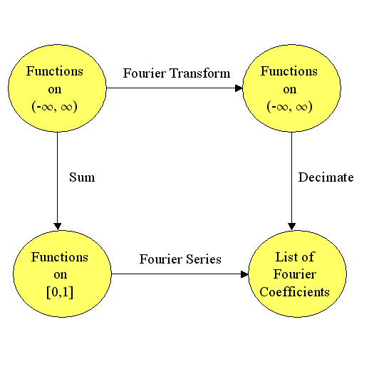
Working on the proof got me thinking about trig functions, modular arithmetic, injective/surjective functions, Fourier transforms, duality, eigenvalues, metric spaces, projections, the Reiz Representation Theorem, Plancherel’s theorem, and numerical integration.

Probability and information theory were largely missing from my week until I stopped by Carl’s house yesterday. He and I got into a discussion about category theory, information theory, and neural networks.  One thing we noticed was that 1-1 functions are the only functions that conserve the entropy of categorical variables. For example, if $X\in\{1,2,3,4,5,6\}$ is a die roll, then $Y=f(X)$ has the same entropy as $X$ only if $f$ is 1-1.  Turns out you can characterize many concepts from Category theory using entropy and information theory.  So we used random variables, probability distributions, histograms, the mean (entropy is the mean value of the log of the probability), standard deviations, the Pythagorean theorem, statistical independence, real numbers, correlation, the central limit theorem, Gaussian Distributions (the number e), integrals, chain rule, spheres, logarithms, matrices, conic sections (the log of the Gaussian is a paraboloid), Jacobians, Bayes Theorem, and compactness.

I almost avoided using the Pigeon Hole Principle, but then Carl argued that we could use the definition of average value to prove Pigeon Hole Principle.  I still don’t feel like I used it, but it did come up in a discussion.

Notably missing from my week were (surprisingly): derivatives, volume formulas (volume of a sphere or cube), Taylor’s theorem, the fundamental theorem of calculus, and about half of the ideas between #63 Boolean algebra and #99 uncountable infinity.

So, it looks like I typically use around 70 ideas from the list each week—more than I thought.


I will probably get back to 2048 stuff later this month and maybe a post on Fourier Transforms.


Have a great day!    – Hein


polarplot2

Equation from Teacher’s Choice

So I have been wanting to understand Category Theory (see [1], [2], [3]) mainly because I thought it would help me understand advanced functional programming in Haskell and because of the book “Physics, topology, logic and computation: a Rosetta Stone” by Baez and Stay (2011).  A number of the constructs in Haskell were derived from Category Theory so that was enough motivation for me to learn it.  But also, monoidal categories are useful in several fields: physics, computer science, pure mathematics, and statistics. The biggest application for me is the idea of generalizing probabilistic graphical models through either Ologs or monoidal categories / tensor networks (see Brendan Fong’s thesis “Causal Theories: A Categorical Perspective on Bayesian Networks“).

To start my investigation of Category Theory, I began with the $20 thin book “Basic Category Theory for Computer Scientists” by Benjamin Pierce (see also the free online version “A taste of category theory for computer scientists” (1988)).

I really enjoyed the book.  Dr. Pierce’s style is a little informal compared to pure math books like Mac Lane’s “Categories for the Working Mathematician” (pdf / Amazon), but I enjoy that more relaxed style of writing when I am first learning a field.

The biggest obstacle for learning category theory is the fact that category theory generalizes a lot of areas of pure mathematics like topology, abstract algebra, and geometry.  It’s hard to generalize before you have examples to generalize, but the examples being generalized in category theory are mostly from higher level mathematics found in senior level undergraduate and graduate level courses. Pierce ameliorates this problem by introducing some of the most basic categories first: sets, ordered sets, partially ordered sets, groups, monoids, vector spaces, measure spaces, topological spaces, proofs, and a simple functional computer language.  He takes the time to explicitly define most of these ideas, so, in theory, you could read this book without a background in theoretical mathematics, but it would be hard.

After defining categories and introducing the most basic categories, Pierce describes and defines the most basic ideas in category theory: subcategories, commutative diagrams, monomorphisms, epimorphisms, isomorphisms, initial/terminal objects, products, coproducts, universal constructions, equalizers, pullbacks, pushouts, limits, cones, colimits, cocones, exponentiation, and closed Cartesian categories. These ideas are spelled out over the thirty pages of chapter one including illuminating homework exercises. The homework exercises varied significantly in difficulty.  Many of the exercises were trivial and there are two or three that I am still working on despite investing several hours of thought.  Generally, I found the exercises to be a bit harder than those in Mac Lane’s book, but Pierce’s book required less of a background in mathematics.  A couple of the exercises were incorrectly stated or impossible.

Chapter two introduced functors, natural transformations, adjoints, and F-algebras. After reading this chapter, I was finally able to understand the definition of monads which are an important part of the computer language Haskell!  Pierce provides many examples of each of these ideas and enjoyable homework exercises to increase understanding.  Pierce’s definition of adjoints is much easier to understand than the standard definitions using counit adjunction or Hom Sets.

The last major chapter concerns applications of category theory to computer science–specifically lambda-calculus and programming language design.  

The first two chapters of the book give a reasonable condensed introduction to category theory for students that have taken a course in abstract algebra.  A course in topology or linear algebra would be another useful prerequisite.  I carried around the light 100 page book for a few months so that I could learn something whenever I had some extra time.  I had hoped that when I had proven that several functors where monads, I would then really understand monads, but a full understanding still eludes me.  Similarly, I have proven that several functor pairs are adjoint, but I still don’t feel as though I understand adjoint functors.  I guess more work and learning are needed.

Have a great year.  –  Cheers, Hein


Orthogonal functions are very useful and rather easy to use.  The most famous ones are sin(n x) and cos(n x) on the interval [$-\pi$, $\pi$].  It is extremely easy to do linear regression with orthogonal functions.

Linear regression involves approximating a known function $f(x)$ as the weighted sum of other functions.  This shows up all the time in various disguises in machine learning:

  • When using AdaBoosting we perform a weighted sum of weak classifiers. 
  • Support vector machines find a linear combination of the features that separates the data into two classes.  
  • Each node in a neural net typically computes a weighted sum of the nodes in the prior layer.

For orthogonal functions, computing the linear regression is simple.  Suppose that the features are $f_1, f_2, \ldots, f_n$ and the functions $f_i$ are orthonormal, then the best approximation of the function $g(x)$ is the same as the solution to the linear regression

$$ g(x) \approx \sum_{i=1}^n \alpha_i f_i(x)$$

where $\alpha_i$ is the “inner product” of $f_i$ and $g$ denoted

$\alpha_i= \langle\;g, f_i\rangle = \int g(x) f(x) w(x) dx.$  (Two function are orthogonal if their inner product (or dot product) is zero.  The set of orthogonal functions $\{f_i\}$ is called orthonormal if $<f_i, f_i>=1$ for all $i$.)  The function $w(x)$ is a positive weight function which is typically just $w(x)=1$.

For example, if we try to approximate the function $g(x)=x^2$ on the interval [-1,1] by combining the features $f_1(x) = 1/\sqrt(2)$ and $f_2(x) = x \sqrt{3 \over 2} $, then

$$ g(x) \approx \sum_{i=1}^n \alpha_i f_i(x)$$

where

$$\alpha_1 = \langle g, f_1\rangle = \int_{-1}^1 g(x) f_1(x) dx =  \int_{-1}^1 x^2 1/\sqrt2 dx = \sqrt{2}/3,$$

$$\alpha_2 = \langle g, f_2\rangle = \int_{-1}^1 g(x) f_2(x)  dx=  \int_{-1}^1 x^2  \sqrt{3/2}\; x dx =0,$$

and the best approximation is then $\sum_{i=1}^n \alpha_i f_i(x) = \alpha_1 f_1(x) = 1/3$.


The other day I needed to do a linear regression and I wanted to use orthogonal functions, so I started by using the trigonometric functions to approximate my function $g(x)$.  Using trig functions to approximate another function on a closed interval like [-1,1] is the same as computing the Fourier Series.  The resulting approximations were not good enough at x=-1 and x=1, so I wanted to change the weight function $w(x)$.  Now assume that $u_1(x), u_2(x), \ldots, u_n(x)$ are orthonormal with the weight function w(x) on [-1,1].  Then

$$ \int_{-1}^1 u_i(x) u_j(x) w(x) dx = \delta_{i,j}$$

where $\delta_{i,j}$ is one if $i=j$ and zero otherwise.  If we make a change of variable $x=y(t)$, then

$$ \int_{y^{-1}(-1)}^{y^{-1}(1)} u_i(y(t)) u_j(y(t)) w(y(t)) y'(t) dx = \delta_{i,j}.$$

It would be nice if

$$(1)\quad w(y(t)) y'(t)=1,$$

because then I could just set $u_i(y(t))$ equal to a trig function and the resulting $u_i(x)$ would be orthonormal with respect to the weight function $w(x)$. Condition (1) on $y$ is really an ordinary differential equation

$$y’ = {1\over{w(y)}}.$$

In order to get a better fit at $x=\pm 1$, I tried two weight functions $w(x) = {1\over{(1-x)(1+x)}}$ and $w(x) = {1\over{\sqrt{(1-x)(1+x)}}}$.  For the former, the differential equation has solutions that look similar to the hyperbolic tangent function. The latter $w(x)$ yields the nice solution

$$y(t) = \sin( c + t).$$

So now if I choose $c=\pi/2$, then $y(t) = \cos(t)$, $y^{-1}(-1) = \pi$, $y^{-1}(1)=0$, so I need functions that are orthonormal on the interval $[-\pi, 0]$.  The functions $\cos(n x)$ are orthogonal on that interval, but I need to divide by $\sqrt{\pi/2}$ to make them orthornormal.  So, I set $u_n(y(t)) = \sqrt{2/\pi}\cos(n\;t)$ and now

$$ \int_{-1}^1 {{u_i(x) u_j(x)}\over {\sqrt{(1-x)(1+x)}}}  dx = \delta_{i,j}.$$

The $u_n(x)$ functions are orthonormal with respect to the weight $w(x)$ which is exactly what I wanted.

Solving for $u(x)$ yields

$$u_n(x) = \sqrt{2/\pi} \cos( n \;\arccos(x)),$$

$$u_0(x) = \sqrt{2/\pi}, u_1(x) = \sqrt{2/\pi} x,$$

$$u_2(x) = \sqrt{2/\pi}(2x^2-1), u_3(x) = \sqrt{2/\pi}(4x^3-3x),\ldots.$$


If you happen to be an approximation theorist, you would probably notice that these are the Chebyshev polynomials multiplied by $\sqrt{2/\pi}$.   I was rather surprised when I stumbled across them, but when I showed this to my friend Ludmil, he assured me that this accidental derivation was obvious.  (But still fun :) )

« Older entries § Newer entries »